How to improve software development process using mathematical models for quality prediction and elements of Six Sigma methodology I. Sinovčić, L. Hribar Ericsson Nikola Tesla R&D Center, Croatia
[email protected],
[email protected] Abstract—In this paper technical cost and financial inputs and outputs will be used as main parameters to propose theoretical model how and where should be main work focus to achieve best financial results. The Six-Sigma methodology was used to prove the models and concept. The paper deals with software quality prediction techniques, different applied models in different development projects and faults existing indicators. Three case studies are presented and evaluated for prediction of software quality in very large development projects within the AXE platform using SIP as a call control protocol in the Ericsson Nikola Tesla R&D.
I.
INTRODUCTION Figure 1. Product Life Cycle
We will present theoretical model to help in decision in which PLCM phase (and sub-phase) is best to invest to achieve goal of minimizing effort and maximizing earnings, based on case studies in handling of SW faults in life cycle of three Ericsson telecom applications, which are using IP call control protocol such as SIP protocol (three big telecom SW packages). Software system functioning in IP network that businesses are increasingly dependent upon was examined. The system is multirelease, in customer operation for over 6 years, structured as single-platform system, and is widely deployed. To be able to improve SW faults handling process, it is a vital to have best understanding of SW faults distribution and associated prediction model. With this knowledge we can then apply improvements techniques more precisely and more effective in advance (proactively) to prevent waste of money and energy. Product Life Cycle Management (PLCM) supports the transformation of customer expectations into complete solutions at the right time with competitive price and performance, satisfying customers and enabling market leadership and financial growth [1]. PLCM flow starts by identifying the possibilities for a product, the demand and the expectations of the market, continues with development and creation of product and in later phases, deployment and maintenance including phase-out or substitution plan. All these management activities are very complex and are using knowledge and experience from many scientific disciplines. In the simple form Product Life Cycle (PLC) is divided in four phases: Select, Create, Manage and Phase out.
From financial point it is always important that product is commercially successful and that product handling effort is minimized with maximized earnings. To have control over PLC phases and sub-phases, controlling points (PDx) are defined and in each point decision is taken about future product related actions. Inside main PLCM process number of processes and procedures existing, precisely defining all process and sub-process steps. Our focus will be on Development process and Modification handling process improvement. II.
SIP PROTOCOL
SIP is an IETF application-layer control protocol that can establish, modify, and terminate multimedia sessions (conferences) such as Internet telephony calls [2]. SIP can also invite participants to already existing sessions, such as multicast conferences. Media can be added and changed to (and removed from) an existing session. SIP transparently supports name mapping and redirection services, which supports personal mobility - clients can maintain a single externally visible identifier regardless of their network location. SIP is not a vertically integrated communications system. It is structured as a layered protocol, which means that its behavior is described in terms of a set of fairly independent processing stages with only a loose coupling between each stage. SIP is a IETF protocol that can be used with other IETF protocols to build complete multimedia architecture. SIP was designed to be a modular part of a larger IP telephony solution and thus functions well with a broad spectrum of existing and future IP telephony protocols.
SIP telephony network is transparently with respect to the Core Network. Traditional telecom services such as call waiting, free phone numbers, etc., implemented in protocols such as SS7 should be offered by a SIP network in a manner that precludes any debilitating difference in client experience while not limiting the flexibility of SIP. III.
QUALITY OF SOFTWARE PRODUCTS
It is always about quality and cost. Or even better, it is always about ratio between quality and cost. Software quality prediction helps minimize software costs. The number of faults in a large software project has a significant impact on project performances and hence is an input to project planning [3], [1], [18], [19]. The ANSI/IEEE definitions for quality control is measuring the quality of a product and the Quality Assurance measures the quality of processes used to create a quality product [16]. IEEE Standard 12207 defines QA this way: "The quality assurance process is a process for providing adequate assurance that the software products and processes in the product life cycle conform to their specific requirements and adhere to their established plans" [4]. The Software Capability Maturity Model version 1.1 states it this way: "The purpose of Software Quality Assurance is to provide management with appropriate visibility into the process being used by the software project and of the products being built". The ISO/IEC 9126 product quality standard [5] is used to categorize the metrics. ISO 9126 (ISO 1991) is called software product evaluation: quality characteristics and guidelines for their use. In this standard, software quality is defined to be “the totality of features and characteristics of a software product that bear on its ability to satisfy stated or implied needs”. Software quality is decomposed into six factors: functionality, reliability, efficiency, usability, maintainability, and portability. The view on the software quality related to this work is presented as anticipated number of software faults in the product life cycle which conform to their specific application requirements, adhere to established projects plans and customer satisfaction with the applications. The motivation for software quality measurement is to understand, control and improve the various quality attributes of the software and the underlying development process. A prerequisite is the definition of the quality attributes and the related measures / metrics. As the quality level of the final product is set at the beginning of the project, a large number of faults can result in project delays and cost overruns [6]. Planning precision and predictability is crucial for the any projects in operations [7], [8]. All stakeholders are dependant on that the project deliver timely according to projects plans. This research work exams the usage of the several mathematical distributions as a models for a software faults prediction techniques. The models are based on statistical and probabilistic approach and identify future research towards a method to select a most suitable prediction technique. Projects used in this paper are developed for AXE platform as a legacy product development environment. The faults in the applications
used for modeling in this paper are presented as a trouble reports. Most of the evaluated projects would have faults distributions very well fitted with mathematical models. Thus Weibull [9], exponential, normal and lognormal distributions were fit to each of the data sets of this study. The models are made in Microsoft Excel [14]. The goodness of fit was determined for each distribution [10]. Finally, details of all statistical analyses are presented in case studies chapter. IV.
MATHEMATICAL MODELS USED IN THE CASE STUDIES
A trouble reports occurrence is the observable event of interest for both maintenance and insurance purposes. The operational definition of a trouble reports occurrence varies across organizations. In this paper, we use the approach to analyze fault occurrences in Ericsson Nikola Tesla R&D organizations using the term TR and the TR inflow over the weeks. The TRs are reports either from the customer, either from the internal verification team, either from ongoing development projects. In general, not every reported TR reports the fault. After analysis some reports are classified as a non-fault but as a misconfiguration or misunderstanding the function [11]. It must be noted that all mathematical distribution presented in this paper used total number of reported faults in time frame without taking care about TR answer code distribution. In the cases where the reported TRs are actually not the faults, the maintenance is negligible (e.g. correcting the documentation, refurnishing the UI or customer documentation) in relation to actual faults which will require the coding of the correction, unit testing, integration testing and regression testing. The purpose of such approach is to find out how many customer reports in total are reported and how many people are needed for the analysis of such customer reports and consequently the application maintenance. This approach is presented as a “the worst scenario for maintenance” because the maintenance efforts or allocated people in the maintenance project will be in the worst case equal to the number of the TRs. In this case applications maintenance efforts will be equal or less than total number of the reported TRs. Software system functioning in IP network that businesses are increasingly dependent upon was examined. This system is multirelease, in customer operation over 5 years, single-platform, and widelydeployed. We have collected data for three different applications, Wln3.0, Wln4.0 and Wln4.1 (three applications in row where the next one is successor of the previous one regarding legacy and functionality). Empirically are addressed two questions that are important for fault occurrence projection: Is there a type of fault occurrence model that provides a good fit to fault occurrence patterns across multiple releases and in many applications as indicated in Figure Figure 2. ? Given such a model, how can model parameters for a new release be extrapolated using historical information? The software development process constantly measure software faults and failures during all development stages in the different projects. The goal is to find fault as much
Application weekly TR rate
Probability density function
0,025
0,02
0,015 Weibull prediction Trouble reports 0,01
0,005
0 1
9
17 25 33 41 49 57 65 73 81 89 97 105 113 Time, weeks
Figure 2. Comparison between Weibull model and real TR data
Our findings support the idea that a common fault occurrence projection method for the one development organization can be used across other development organizations for similar or even different development styles. A. Weibull model distribution The Weibull distribution is by far the world’s most popular statistical model for life data. Weibull distribution is also used in many other applications, such as weather forecasting and fitting data of all kinds. Comparison between Wln3.1 Wln4.0 and Wln4.1 Weibull pdf
Weibull probability density function
0,016 0,014 0,012 0,01
Wln4.1
0,008
Wln4.0
Correlation coefficient (cc) and chi-square statistics (Χ²) are also shown in the Table 1 to evaluate proposed model. It must be noted that the expected frequency is for some cases below 5 (some statisticians suggest that each expected frequency should be greater than or equal to 5 for chi-square test to be valid) but even with this limitation the results are very much the same (cc and chi-square statistics). A change in the scale parameter η has the same effect on the distribution as a change of the abscissa scale. In the observing applications it can be seen that value of η is decreasing while the β and γ are kept very much the same. Since the area under a Probability Density Function (pdf) curve is a constant value of one, the "peak" of the pdf curve will also increase with the decrease of η. The faults distribution gets pushed in towards the left (i.e. towards its beginning or towards 0 or γ), and its height increases, as indicated in Figure 4. The parameter η has the same units as T, such as hours, miles, cycles, actuations, etc. B. Lognormal model distribution The lognormal distribution is commonly used to model the lives of units whose failure modes are of a fatigue-stress nature. Since this includes most, if not all, mechanical systems, the lognormal distribution can have widespread application. Comparison between Wln3.1 Wln4.0 and Wln4.1 lognormal pdf 0,02 Lognormal probability density function
as possible earlier and to fixed them and to save hours and money for the organization.
0,018 0,016 0,014 0,012
Wln4.1
0,01
Wln4.0
0,008
Wln3.1
0,006 0,004 0,002
Wln3.1
0,006
0 0,00
50,00
100,00
0,004
150,00
200,00
Time, weeks
0,002
Figure 4. Lognormal model measurement
0 0,00
50,00
100,00
150,00
200,00
Time, weeks
TABLE II. Figure 3. Weibull model measurement
TABLE I. Wln3.1 Wln4.0 Wln4.1
β 1,6824726530 1,4546092221 1,7496187407
WEIBULL DISTRIBUTION PARAMETERS η 76,3333878248 55,5971983756 53,9475173776
γ 0,0000000000 0,0000000000 0,0000000000
cc 0,9876931049 0,9866774212 0,9714454901
Χ² 0,660681736 0,353361177 0,576401149
Among all statistical techniques it may be employed for engineering analysis with smaller sample sizes than any other method. The Weibull distribution was first published in 1939, over 60 years ago and has proven to be invaluable for life data analysis in aerospace, automotive, electric power, nuclear power, medical, dental, electronics, and every industry. Data obtained in 0are Weibull parameters η = scale parameter, β = shape parameter (or slope) and γ = location parameter.
Wln3.1 Wln4.0 Wln4.1
LOGNORMAL DISTRIBUTION PARAMETERS
Sigma T' 0,767425128 0,935035201 0,792243527
u' 3,992593618 3,622318404 3,659258519
cc Χ² 0,978963033 10,88787438 0,927482871 0,894285681 0,895150192 2,5443787047
Consequently, the lognormal distribution is a good companion to the Weibull distribution when attempting to model these types of units. As may be surmised by the name, the lognormal distribution has certain similarities to the normal distribution. A random variable is lognormal distributed if the logarithm of the random variable is normally distributed. Because of this, there are many mathematical similarities between the two distributions. The lognormal distribution is a distribution skewed to the right. The pdf starts at zero, increases to its mode, and decreases thereafter. The parameter u', in terms of the logarithm of the T's is also the scale parameter, and not the location parameter
as in the case of the normal pdf. The parameter Sigma T', or the standard deviation of the T's in terms of their logarithm or of their T, is also the shape parameter and not the scale parameter, as in the normal pdf, and assumes only positive values. In the observing applications it can be seen that value of degree of skewness (Sigma T') decreases, for a given u' as indicated in the 0 It means that for the very much the same value of u' (Wln4.0 and Wln4.1), the pdf will gets pushed in towards the left (i.e. towards its beginning or towards 0) because Sigma T' for Wln4.0 is much higher than for Wln4.1 as indicated in Figure 4. The parameter u', in terms of the logarithm of the T's is also the scale parameter, and not the location parameter as in the case of the normal pdf. The parameter Sigma T', or the standard deviation of the T's in terms of their logarithm or of their T', is also the shape parameter and not the scale parameter, as in the normal pdf, and assumes only positive values. C. Normal model distribution The normal distribution, also known as the Gaussian distribution, is the most widely-used general purpose distribution. Comparison between Wln3.1 Wln4.0 and Wln4.1 normal pdf
scale parameter of the normal pdf. In the observing applications it can be seen that for the very much the same value of u as Sigma T decreases, the pdf gets pushed toward the mean, or it becomes narrower and taller (Wln4.0 and Wln4.1 applications) as indicated in the 0As Sigma T significantly increases (Wln3.1 application) the pdf spreads out away from the mean, or it becomes broader and shallower as indicated in Figure 5. D. Exponential model distribution The exponential distribution is a commonly used distribution in reliability engineering. Mathematically, it is a fairly simple distribution, which many times lead to its use in inappropriate situations. It is, in fact, a special case of the Weibull distribution where β - 1. The exponential distribution is used to model the behavior of units that have a constant failure rate (or units that do not degrade with time or wear out). As mentioned before, the primary trait of the exponential distribution is that it is used for modeling the behavior of items with a constant failure rate. It has a fairly simple mathematical form, which makes it fairly easy to manipulate. Unfortunately, this fact also leads to the use of this model in situations where it is not appropriate. However, some inexperienced practitioners of reliability engineering and life data analysis will overlook this fact, lured by the siren-call of the exponential distribution's relatively simple mathematical models. Comparison between Wln3.1, Wln4.0 and Wln4.1 Exponential pdf
0,016 0,014
0,03
0,012
Wln4.1
0,01
Wln4.0
0,008
Wln3.1
0,006 0,004 0,002 0 0,00
50,00
100,00
150,00
200,00
Time, weeks
Exponential probability density function
Normal probability density function
0,02 0,018
0,025 0,02 Wln4.1 0,015
Wln4.0 0,01 0,005 0 0,00
Figure 5. Normal model measurement
TABLE III. Wln3.1 Wln4.0 Wln4.1
Sigma T 47,8836589460 27,4369890508 20,9782930940
cc 0,9547806691 0,9892864686 0,9877047462
50,00
100,00
150,00
200,00
Time , weeks
Figure 6. Exponential model measurement
NORMAL DISTRIBUTION PARAMETERS u 68,9681274900 48,3263506064 45,9500805153
Wln3.1
Χ² 0,9003004420 0,3192545587 0,4847624232
It is for this reason that it is included among the lifetime distributions commonly used for reliability and life data analysis. There are some who argue that the normal distribution is inappropriate for modeling lifetime data because the left-hand limit of the distribution extends to negative infinity. This could conceivably result in modeling negative times-to-failure. However, provided that the distribution in question has a relatively high mean and a relatively small standard deviation, the issue of negative failure times should not present itself as a problem. Nevertheless, the normal distribution has been shown to be useful for modeling the lifetimes of consumable items. The standard deviation, Sigma T, is the
TABLE IV. Wln3.1 Wln4.0 Wln4.1
EXPONENTIAL DISTRIBUTION PARAMETERS Lambda 0,0210599290 0,0262913928 0,0266803058
Χ² cc 1,2335074444 -0,9666281337 0,8438540990 -0,9129510946 1,4867356755 -0,8596544792
The exponential pdf has no shape parameter, as it has only one shape. The exponential pdf is always convex and is stretched to the right as λ decreases in value as indicated in Figure 6. The value of the pdf function is always equal to the value of λ at T = 0 (or T = γ). The location parameter, γ, if positive, shifts the beginning of the distribution by a distance of γ to the right of the origin, signifying that the chance failures start to occur only after γ hours of operation, and cannot occur before this time. The one-parameter exponential reliability function starts at the value of 100% at T = 0, decreases thereafter
monotonically and is convex. The two-parameter exponential reliability function remains at the value of 100% for T = 0 up to T = γ, and decreases thereafter monotonically and is convex as indicated in the 0The reliability for mission duration of , or of one MTTF duration, is always equal to 0.3679 or 36.79%. This means that the reliability for a mission which is as long as one MTTF is relatively low and is not recommended because only 36.8% of the missions will be completed successfully. In other words, of the equipment undertaking such a mission, only 36.8% will survive their mission. V.
VI.
DEVELOPMENT AND FAULT HANDLING PROCESS
Development process is connected to Select and Create parts of PLCM while Fault Handling process is connected to Create and Manage PLCM parts, Figure 7. It is visible that there is a strong interaction between these processes, especially in area of product technical characteristics but also very much in area of cost and overall financial effectiveness.
DISCUSSION ON THE CASE STUDIES RESULTS AND IMPLICATIONS ON THE PROJECT MANAGEMENT
The presented results in this case studies shows that the mathematical models are suitable and are indeed a good match for the distribution of TRs over time distribution. Estimation of parameter for mathematical models is necessary for accurate prediction of expected number of TRs over a period of time based on customer service requests and operating conditions for developing cost effective maintenance projects. The case studies results show that the correlation coefficients for all mathematical models are very high and determine the goodness of fit. Further investigation on large sample of applications is needed to see are there any inconsistency between cc and chi-square statistics in correlation to goodness of fit. Weibull model is the preferred one for Wln3.1 application among different models due to the fact that the correlation coefficient was highest 0.987 for all observed applications and chi-square statistic is the lowest one. For Wln4.0 Weibull and Normal models are very close to each other. Finally, for Wln4.1 Normal model is slightly better than Weibull model (the highest cc=0.987 and lowest chi-square statistic 0.48). The last but not the least is the impacts of the results and relationship for the project management. The software faults prediction must be used in the project planning and resource allocation within the different project stages. The presented results imply that the resource allocation should take into consideration resource allocation and the faults distribution in the previous projects. Furthermore, resource planning is in direct relationship with the size of the project. The consequence of the bad resource planning is directly connected with the size of the project. Consequences on the organization depend on the project size and project complexity which means that the bigger project will have the bigger consequences on the organization. If the project was bad planned or if the quality of the software is not good enough, originally planned project activities and project commitments will not be kept. To overcome these situation project managers often requires from organization management more people to be added into the project. Adding more people to a late project or to the project with the quality problems makes it only later with questionable quality [15]. At the same time, organization has definite number of available people which leads us to the domino effect with the other projects and their commitments.
Figure 7. SW development process overview
Development process is almost always using Project process as main sub-process and is divided in phases. Common naming for the check points beetwen these phases is either TG (tollgates) or MS (milestones) referring to specific moments/status in project life. TGs and MSs are precisely defined inside project process, with clear managerial, technical and financial activities and responsibilities. Fault handling process is using parts of development process but also number of specific routines for fixing the faults created during development process as indicated on Figure 8. Sole purpose of Fault handling process is to be used for fixing faults. Faults are grouped in two basic groups: Faults created due to faulty product design Faults created due to development process faults In either case Fault handling process is used to fix faults and bring out fault-free product. It is clear that cost issue is very much important for Fault handling and decreasing this cost is always in high focus of any development organization.
Customer
Reception
PreAnalysis
Analysis
Answer handling
Closure
Problem
Customer
Solution
Figure 8. Fault handling process overview
Fault reporting can be directly from customer, but also from sales or packaging organization inside company itself, but most importantly number of faults can come from company’s development organization, when released products are used in new developed applications.
VII. COST ANALYSIS STUDY Although reported faults can come from various inputs, we will not consider this difference and only important input data for this analysis is volume and type of received faults per PLC (product life cycle) phase and sub-phase At Ericsson there are very sophisticated tools for collection, analysis and resolving of received faults [12]. Using these tools we have collected data for Wln3.0, Wln4.0 and Wln4.1 applications, Figure 9.
Figure 9. Fault/Cost distribution per phases
Fixing of fault in Basic and Function test is three times less expensive than in Design follow-up phase and four times less expensive than in full product use (Maintenance phase). It is clear that fixing of the fault is much cheaper if it is done as early as possible. So in parallel with main goal which is fault free design and product, it is also very much important to move fault detection and solution as early as possible to save as much money as possible Six Sigma methodology is used to improve fault finding and fixing in very early phases of product development and usage (early phases of PLC) [13]. VIII. SIX SIGMA METHODOLOGY OVERVIEW Six Sigma is a worldwide well-proven change engine. The result is often improved cost savings, increased quality, higher customer satisfaction, shortened lead-times or boosted efficiency.
Chang e Change Managem ent Management
Successful Deployment Results Results
Methodology Methodology
Figure 10. Basic triangle for successful improvements deployment
It is a systematic methodology to home in on the key factors that drive the performance of a process, set them at the best levels, and hold them there for all time. It is also a kind of management philosophy that can radically change the way you treat mistakes in the workplace and is
focused on eliminating these mistakes, teaching personnel how to improve performance. The Greek letter Sigma, used mathematically to designate standard deviation, is the measure used to determine how good or bad the performance of a process is. In other words, it represents how many mistakes a company commits while accomplishing its tasks. On the other hand, the Six in “Six Sigma” represents the levels of perfection each company attains. One Sigma equates to about 700,000 defects per million opportunities, or doing things right 30% of the time. Two Sigma is better with a little over 300,000 mistakes per million opportunities. Most companies operate between Three and Four Sigma, which means they make between approximately 67,000 and 6,000 mistakes per million chances, respectively. If you’re operating at 3.8 Sigma, that means you’re getting it right 99% of the time. The traditional approach to Six Sigma involves the steps that focus on discovering customers’ critical requirements, developing process maps, and establishing key business indicators. After these steps are completed, the business moves on to review its performance against the Six Sigma standards of performance and takes actions to realize virtual performance. The approach, used by Motorola during the first 5 years, requires leadership and managerial staff to undergo extensive training for change management supported The new approach to Six Sigma, called the Breakthrough approach, captured the Motorola methods and packaged them in the Define, Measure, Analyze, Improve, and Control (DMAIC) methodology. The Breakthrough approach consists of management involvement, organizational structure to facilitate the improvement, customer focus, opportunity analysis, extensive training, and reward and recognition for successful problem solving. Its benefits include the standardization of the methods, global adaptation of the methodology, and commercialization of Six Sigma [17],[20], [21]. The project-level implementation relies on the DMAIC methodology for improvements and IDDOV (Identify, Define, Design, Optimize, and Verify) for design activities. Extensive training is standard part of competence buildup for champions and sponsors, Black Belt and Green Belt candidates, and employees. The training for champions and sponsors includes an understanding of the need for Six Sigma, Six Sigma’s benefits, the rollout plan, the working of Six Sigma projects, the roles and responsibility of all employees (including executives), and an overview of the DMAIC methodology. IX.
DMAIC PROJECT STRUCTURE PROPOSAL
For this exercise we are taking assumption that total number of incoming faults is same prior and after improvements, although generally with proposed improvements total number of faults should also be reduced. Main goal is to reduce fault slip through effect, and by doing that decrease costly fault fixing in later PLC (product life cycle) phases.
B. Measure To be able to come to right conclusion, we should collect faults reported in all PLC phases and sub-phases with additional fault data included like: Gravity of fault Type of fault (SW, HW, documentation, coding, requirements, etc) Repetition of the fault Market specific info Phase/sub-phase where the fault is found There is a number of parameters available per each fault reported and using simple Cause and Effect matrix analysis and later Process Failure Mode and Effect analysis (FMEA) table we have narrowed input data to only two ‘Phase/sub-phase info’ and ‘Type of the fault’ as most important for this analysis. Known Six Sigma equation Y = f(X1,X2,..., Xn) to describe process performance is simplified to Y = f(X1,X2), where Y is process result and Xn are number of process inputs. C. Analyze Our focus in this case is on process effectiveness side with question to be answered: How may fault found in later PLC phases be able to have been found during earlier verification activities (earlier PLC phases)? Achieving process more effective will also result in increased process efficiency as well. Pareto chart of Fault types 120
100
Percent
80
60
• • •
Type C (possible to detect earlier using better detection tools) Type D (possible to detect earlier with more detailed testing) Other (undefined possibility)
It is clear that in case of type C and type D we can improve fault detection and resolution by improving Software Development process in domain of testing and testing tools. For B type, specific setup is needed and generally it is not process dependent. Simulation that ~5% faults have been earlier detected is shown in Figure 12. Simulation results for Wln3.1, Wln4.0 and Wln4.1 using Weibull 0,016 Weibull probability density function
A. Define As indicated in table in Figure 9. , problem can be defined as ‘too many faults find too late’. So if the goal is quantified as 5% increase in cost efficiency, than total cost for each application should be decreased by 5%. If total expected number of the faults is the same, focus should be on redistribution of these faults, by redistribution of effort in different process phases.
0,014 0,012 Wln4.1 imp 0,01
Wln4.0 imp Wln3.1 imp
0,008
Wln4.1 Wln4.0
0,006
Wln3.1 0,004 0,002 0 0,00
50,00
100,00
150,00
200,00
Time, weeks
Figure 12. Simulation results
This simulation is very useful in prediction of application fault density behavior (fault distribution) if we put more effort to Function test and Network Integration test (NIV). Our planning in this case can include improved fault distribution and utilization of needed resources can be adjusted accordingly.
X.
PROCESS IMPROVEMENT PROPOSAL
D.
Improve Software development process is complex multidimensional process, but for this exercise we will simplify model, considering only two basic dimensions, functional/technical dimension from pre-study, feasibility, design activities, over to integration and verification of SW product (NIV test), and organizational/operational dimension with focus on SW development line and project organization. This process structure is in simple form shown on Fig13 [22].
40
20
0 Type A
Type B
Type C
Type D
Other
Fault types
Figure 11. Pareto chart of fault types
Pareto chart (Figure 11. ) is used to analyze fault data. By using known ‘Phase/sub-phase info’ and ‘Type of the fault’ data, faults are classified into five groups: • Type A (not possible to detect earlier) • Type B (possible to detect earlier for specific customer setups) Figure 13. Process improvement proposal
Function test and Integration and Verification test must be improved to catch faults early enough, which would otherwise slip through to later PLC phases. Further detail analysis is needed to investigate detail direction of improvements; either it is more time consuming needed for these critical PLC phases or strictly process element improvements or combination of two. Our project is ongoing with this investigation and work on it. Control Big size telecom applications like Wln3.1, Wln4.0 or Wln4.1 last over a year and feedback control is rather difficult if we are waiting for complete application results. It is more logical to use elements of application that can be verified against proposed improvement and tracked to get results and conclusions on process behavior. From these partial control activities, we can influence overall process performance and later measure complete application output against expected outcome.
REFERENCES [1] [2] [3]
E.
XI. CONCLUSION Quality is something very hard to define, but it is a measure about how confident is user of the services in operator/vendor. It is always about quality and how the product behaves during live operations. However, faultfree product most likely will not be affordable. Without some balance to the interests of the Quality assurance function, it can become too large. These are the influences of the classic market-share dilemma. There is no perfect quality; only good enough. Prediction of data behavior, such as faults in telecom application, is very valuable and has high cost saving potential. If that methodology is joined with process improvements, creating methodology for prediction of fault distribution into new improved process, it can help us in understanding how good our improvements are early enough. It’s time that we developed approaches and methodologies that apply to the whole craft, not just to space missions, medical devices, or academic experiments. It must be stressed again, quality is very important especially today when we have huge competitions on the market. We are witnesses that some of the big vendors with the long history are not very successful today on the market. On the other hand, some new players are very eager to grab market cake. Who will win in this competition? Manufacturers with good enough and first time right quality products. And how can we reach the good enough quality products?
[4]
[5] [6]
[7]
[8]
[9] [10] [11]
[12] [13]
[14] [15]
[16] [17] [18] [19] [20] [21]
[22]
***, “Product Life Cycle Management”, Internal Ericsson documentation, 2008 RFC 3261, Session Initiation Protocol (SIP) Miroslaw Staron, Wilhelm Meding, “Predicting Short-Term Defect Inflow in Large Software Projects – An Initial Evaluation”, 11th International Conference on Evaluation and Assessment in Software Engineering, EASE 2007. James Bach, “Good Enough Quality: Beyond the Buzzword”, Software Realities, 1997.IEEE standard for a software quality metrics methodology, IEEE Std 1061-1998, Dec 1998. ISO/IEC 9126-1:2001 --- Software engineering -- Product quality -- Part 1: Quality model, 2001. Tony Rosqvist, Mika Koskela, Hannu Harju, “Software quality evaluation based on expert judgement”, Software Quality Journal, 11, 39-55, 2003 Lovre Hribar, Sanja Bogovac, Zdenko Marinčić, “Implementation of Fault Slip Through in Design Phase of the Project”, 31. International Conference, MIPRO 2008. Lovre Hribar, “Usage of Weibull and other models for software faults prediction in AXE”, 2008. International Conference on Software, Telecommunications & Computer Networks, SoftCOM 2008. Abernethy R.B., “The New Weibull handbook”, Gulf publishing Co., PO. Box 2608, Dept. AT Houston Texas, 1994. Edgeman, R.L., “Correlation Coefficient Assessment of NPPs”, Reliability Review, Vol. 10, (14-16), 1990. Lovre Hribar, “Software Component Quality Prediction in the Legacy Product Development Environment Using Weibull and Other Mathematical Distributions”, 2009. International Conference on Software, Telecommunications & Computer Networks, SoftCOM 2009 http://mhweb.ericsson.se/index2.html Thomas Pyzdek, The Six Sigma Handbook Revised and Expanded A Complete Guide for Green Belts, Black Belts, and Managers at All Levels, © 2003 by The McGraw-HIll Companies, Inc., 0-07141596-3 http://office.microsoft.com/enus/excel/FX100487621033.aspx Lovre Hribar, “First Time Right in AXE using One track and Stream Line Development”, 32. International Conference, MIPRO 2009. www.asq.org http://sixsigmatutorial.com/ http://www.apmforum.com/emerald/tqm-asia-research.htm http://www.hkbu.edu.hk/~samho/tqm/tqmex/model.htm http://www.isixsigma.com/tt/ Galinac, Tihana, Car Zeljka: Software Verification Process Improvement Proposal Using Six Sigma, LNCS Vol. 4589 Springer (2007), pp. 51-64. Galinac, Tihana: Improving Software Development Efficiency by Managing Early Verification Process, PhD Thesis, Zagreb: Faculty of electrical engineering and computing