Paper 261-27
How to Use SAS for Logistic Regression with Correlated Data Oliver Kuss, Institute of Medical Epidemiology, Biostatistics, and Informatics, Halle/Saale, Germany
ABSTRACT Many study designs in applied sciences give rise to correlated data. For example, subjects are followed over time, are repeatedly treated under different experimental conditions, or are observed in logical units (e.g. clinics, families, litters). Statistical methods for regression analysis for this kind of data with continuous responses are quite established and the SAS system offers a variety of procedures (GLM procedure, MIXED procedure) for analysis. For discrete responses, however, we have to face a greater mathematical complexity and statistical analysis is not that straightforward any longer. We show the different options that the SAS system offers for the analysis of binary responses with correlated data (GENMOD procedure, %GLIMMIX, %NLINMIX, NLMIXED procedure, PHREG/LOGISTIC procedure and Meta-Analytic methods), investigate their statistical properties, and illustrate them by an example of a multicenter study. We conclude that it is difficult to give general recommendations which of the methods to use because this depends on the data at hand and on the desired interpretation of parameters, but in our data set we feel most comfortable with the results from the NLMIXED and the PHREG/LOGISTIC procedure.
INTRODUCTION The logistic regression model has become the standard analyzing tool for binary responses in a variety of disciplines. Reasons for this are: ease of interpretation of parameters as adjusted odds ratios, possibility of calculating prognoses for the event of interest, and availability of standard software. The LOGISTIC procedure is the standard tool in SAS software for fitting logistic regression models, but solutions with the GENMOD, the PROBIT, or the CATMOD procedure are also possible. A crucial point in standard logistic regression analysis is that observations are independent of one another and it is known that violations of this assumption result in invalid statistical inference. However, many study designs in applied sciences give rise to correlated data. For example, subjects are followed over time and responses are assessed at different time points, are repeatedly treated under different experimental conditions, or are observed in logical units (e.g. clinics, families, litters). In the following we illustrate the different options that SAS software offers for the analysis of binary responses with correlated data (GENMOD procedure, %GLIMMIX, %NLINMIX, NLMIXED procedure). We show that each of them estimates parameters from one of two different statistical models and comment on the interpretation of parameters and the statistical properties of the methods involved. The models and the estimation procedures are illustrated by an example of a multicenter randomized controlled clinical trial. THE DATA The data set that we use to explain the various procedures was originally reported by Beitler/Landis, 1985, and was also used by Wolfinger, 1999, to introduce the new NLMIXED procedure. The data have been collected in a multicenter randomized controlled clinical trial conducted in eight different clinics. The purpose of the study was to assess the effect of a topical cream treatment compared to no treatment on curing nonspecific infections. In each of the eight clinics (clinic), the number of treated (n) and the
number of successfully cured persons (x) were recorded for treatment (treatment=1) and control (treatment=0). The SAS data set is the following: data infection; input clinic treatment x n; datalines; 1 1 11 36 1 0 10 37 2 1 16 20 2 0 22 32 3 1 14 19 3 0 7 19 4 1 2 16 4 0 1 17 5 1 6 17 5 0 0 12 6 1 1 11 6 0 0 10 7 1 1 5 7 0 1 9 8 1 4 6 8 0 6 7 run; A CRUDE ANALYSIS A first preliminary analysis to assess the treatment effect will maybe ignore the fact that the data were observed in different clinics and collapse the data in a single 2x2-table. A suitable measure for treatment effect in this case is the odds ratio and the FREQ procedure can be used to achieve an estimator. Some small data manipulation (actually writing each person with its response (cure) in a single line) has to precede the analysis (the variable status will be needed in a later analysis): data infection2(drop=i); set infection; do i=1 to n; if i x then cure=0; status=2-cure; output; end; run; proc freq data=infection2; tables treatment*cure / relrisk; run; This analysis yields an estimated odds ratio [with 95%-CI] of 1.498 [0.915; 2.452], that means the odds for curing the infection is roughly 50% higher in the treatment compared to the control group. However, proceeding this way completely ignores the fact that the study was undertaken in several clinics and we might suspect that different features of them (personnel, environment, typical population of patients) might influence the treatment effect in the individual clinic. Note that this also implies that there is a correlation of patients within individual clinics. In a clinic with high treatment effect many patients will be cured and a cure in a single patient will be accompanied with a higher probability by a cure of another patient from the same clinic.
Because both, fixed effects (here: treatment) and random effects (here: the intercept) are combined in the model, these models are also sometimes called mixed effects models.
THE LOGISTIC REGRESSION MODEL WITH CORRELATED DATA In the following section we show several methods for analysing the described data set with SAS software that explicitly account for the correlation between patients in the different clinics. First, we introduce some notation: Let Yij, i=1,..., n, j=1,...,ni, denote whether patient j in clinic i was cured (Yij = 1: yes, Yij = 0: no) and xij whether patient j in clinic i was in the treatment or in the control group (xij = 1: treatment, xij = 0: control). The response Yij is assumed to follow a Bernoulli distribution where the probability of cure is denoted by pij, that is pij = P(Yij = 1) and this also equals the expected cure E(Yij) = pij.
THE GENMOD PROCEDURE The GENMOD procedure is the SAS procedure for fitting Generalized Linear Models, a class of regression models for univariate responses with density from an exponential family (McCullagh/Nelder, 1989) which includes, besides others, linear, logistic and Poisson regression. Since SAS Version 6.12 the GENMOD procedure also allows the modelling of correlated data via the REPEATED-Statement where the implemented estimation method is the GEE (=Generalized Estimation Equation) of Liang/Zeger, 1986. Thus, this procedure can be used to fit our data set in the context of marginal models and the following call of the GENMOD procedure realizes this:
MARGINAL VERSUS RANDOM EFFECTS MODELS The are two large families of statistical models that account for the correlation in a different style and whose estimated parameters have different intepretations, marginal models and random effect models (Diggle, Liang, Zeger, 1994). In a marginal model the effect of treatment is modelled separately from the within-clinic correlation. A marginal logistic regression model for our data set is given by:
proc genmod data=infection2 descending order=data; class treatment clinic; model cure=treatment / d=bin link=logit; repeated subject=clinic / type=cs; estimate "treatment" treatment 1 -1 / exp; run;
logit(pij) = b0 + btreat xij Var(Yij) = pij (1- pij) Corr(Yij,Yik) = α
We have to specify the logistic regression model from the familiy of Generalized Linear Models by the D=- and the LINK=-Option in the MODEL-Statement. Invoking the REPEATED-Statement calls for the GEE analysis and the TYPE=CS-Option specifies the desired within-clinic correlation matrix. The ESTIMATE-Statement delivers the estimated odds ratio for the treatment effect.
The interpretation of the parameters is analogous to the standard logistic regression model. The transformed regression coefficient exp(btreat) is the odds for cure for a treated patient divided by the odds for cure in a patient from the control group. However, in this model we adjusted for the correlation between patients from the same clinic and we assumed that this correlation is identical for every two patients from the same clinic. Of course, patients from different clinics are considered to be independent. The interpretation of the parameter does not depend on the respective clinic but rather is valid for the whole population of clinics in the study and actually averages the treatment effect across the clinics. This is why the parameters from marginal models are sometimes called population-averaged parameters.
THE %GLIMMIX MACRO The %GLIMMIX macro was written by Russ Wolfinger from SAS Institute and is available from the SAS homepage (http://ftp.sas.com/techsup/download/stat/glmm800.html, please note that we refer to the most recent version which requires Version 8). The macro is designed for the analysis of Generalized Linear Mixed Models (GLMM), and as our random effects logistic regression model is a special case of that model it fits our needs. An overview about the macro and the theory behind is given in Chapter 11 of Littell et al., 1996. Briefly, the estimating algorithm uses the principle of quasi-likelihood and an approximation to the likelihood function of the model that results in an iterative procedure repeatedly fitting a linear mixed model to a pseudo response. The macro was originally written to estimate the pseudo-likelihood function of Wolfinger/O’Connell, 1993, which extended the penalized quasi-likelihood approach of Breslow/Clayton, 1993, by estimating an additional overdispersion parameter. A third approach to fitting GLMM, the so called marginal quasilikelihood approach (MQL, Breslow/Clayton, 1993), is a simplification of the other two approaches that uses a cruder Taylor series expansion to define the pseudo response. The MQL is no longer recommended because it has shown deficiencies in estimating the variance parameters of the random effects, at least in some situations (Brown/Prescott, 1999). The following SAS code fits our data set with the %GLIMMIX macro in the context of Generalized Linear Mixed Models:
In a random effects model it is assumed that there is natural heterogeneity across the clinics and that this heterogeneity can be modelled by a probability distribution (in our case the normal distribution) which means that the regression coefficients vary from one clinic to another. By using this approach the correlation between patients from the same clinic arises from their sharing specific but unobserved properties of the respective clinic. A random effects logistic regression model (more specifically: a random intercept logistic regression model because the intercept is the only random parameter) for our data set is given by: logit(P(Yij = 1) | ui) = b0 + btreat xij + ui with ui ~ N(0,ν2). We assume further that, given ui, the responses from the same clinic are mutually independent, that is the correlation between patients from the same clinic is completely explained by them having been treated in the same clinic. By including only the random intercept ui but keeping the treatment effect fixed we assume that there is a single individual cure probability in each clinic but the effect of treatment is identical across the clinics. This single individual cure probability is the reason why parameters from random effects models are also called subject-specific parameters The interpretation of parameters is also analogous to the standard logistic regression model. The transformed regression coefficient exp(btreat) is the odds for cure for a treated patient compared to a control group patient. The variance ν2 measures the degree of heterogeneity in the probability of cure that can not be explained by treatment.
%include "...\glmm800.sas"; %glimmix(data=infection2, stmts = %str( class clinic; model cure = treatment / solution cl; random clinic; parms (0) (1.0) / EQCONS=2; ), error=binomial,
2
link=logit, procopt=order=data );
derivs=%str( d_b0 = num /(den*den); d_b_treat = treatment*num /(den*den); d_u = num /(den*den); ), stmts = %str( class clinic; model pseudo_cure= d_b0 d_b_treat / noint solution cl; random d_u / subject=clinic cl solution; ), procopt=empirical, expand=zero /* This line for Method 1 */ expand=eblup /* This line for Method 2 */ ); run;
run; The model is actually defined in SAS PROC MIXED syntax and the relevant statements are given in the STMTS argument. Using the EQCONS=2-Option in the PARMS-Statement fixes the overdispersion parameter at the given value of 1 and thus requests the estimation of the penalized quasi-likelihood model of Breslow/Clayton, 1993. Leaving out the EQCONS=2-Option gives the pseudo-likelihood estimates of Wolfinger/O’Connell, 1993. The ERROR=BINOMIAL and LINK=LOGIT arguments define the logistic regression model and PROCOPT=ORDER=DATA ensures the proper ordering of the treatment effect. THE %NLINMIX MACRO The %NLINMIX macro was also written by Russ Wolfinger from SAS Institute and is available from the SAS homepage (http://ftp.sas.com/techsup/download/stat/nlmm800.html, please note that we refer to the most recent version of the macro which is even more important as with the %GLIMMIX macro because there were substantial syntax changes to Version 8). The %NLINMIX macro is actually designed for the analysis of nonlinear mixed models, but a simple transformation of the model equation shows that we can write our random effects logistic regression model as a nonlinear model:
* Code for Estimation method 3; %include "...\nlmm800.sas"; %nlinmix(data=infection2, model = %str( num = exp(b0 + b_treat*treatment); den = 1 + num; predv = num/den; weight = 1/predv; ), parms = %str(b0=-0.7142 b_treat=0.404), derivs = %str( d_b0 = num /(den*den); d_b_treat = treatment*num /(den*den); ), stmts = %str( class clinic; model pseudo_cure= d_b0 d_b_treat / noint solution cl; repeated / sub=clinic type=cs; weight weight; ), procopt=empirical ); run;
Yij = expit(b0 + btreat xij +ui) + εij with ui ~ N(0,ν2), εij ~ N(0,σ2), ui and εij uncorrelated, and expit(a)=exp(a)/(1+exp(a)). The necessity of including the measurement error εij in the model equation arises from the fact that we now directly model the response Yij and no longer its expected value. A thorough description of the %NLINMIX macro, the implemented methods, and their properties is given in several articles by Wolfinger and co-authors (Litell et al., 1996 (Chap. 12), Wolfinger, 1997, Wolfinger/Lin, 1997). Shortly, the %NLINIMX macro provides (at least) three different methods of parameter estimation. The first two estimation methods are based on a Taylor series expansion around values for the random effect parameters where the first method expands around the zero vector and the second around the best empirical linear unbiased predictor (EBLUP) of the random effects. Both approximations result in algorithms that iterate linear mixed models for suitably defined pseudo responses. Theoretically, the EXPAND=EBLUP-method gives more reliable results because it uses a more accurate Taylor series expansion (Wolfinger, 1997), whereas the EXPAND=ZERO-method is considered to be more stable and less time consuming. There are close connections to several other methods of parameter estimation in nonlinear mixed effects models (Wolfinger/Lin, 1997). The third method, finally, is a refined GEE estimation, that is, it actually fits a marginal model. To be concrete, it extends the fitting algorithm used in the GENMOD procedure by using a quadratic instead of a simple method of moment estimation equation for the correlation parameters (Davidian, 2001). The following SAS code fits the described models:
The macro code is rather technical, and the instructions how to define the correct model are given in the header of the macro. The nonlinear model is coded by standard SAS programming language with the MODEL argument, the nonrandom parameters are given with suitable starting values in the PARMS argument, derivations of all model parameters are given in the DERIVS argument, and in the STMTS argument the model is defined in SAS PROC MIXED syntax. Note the differences between the random effects models in the first %NLINMIX call and the marginal model in the second call: the marginal model uses the REPEATED-Statement instead of the RANDOM-Statement in the STMTS argument, and there is no reference to the random effect u. THE NLMIXED PROCEDURE The statistictical methods used in the %GLIMMIX and in the %NLINMIX are only approximative as they do not maximize the likelihood of the model directly but only approximations of it. This is necessary because the likelihood of the model incorporates untractable integrals that can be calculated directly only in special cases or with considerable effort. The new NLMIXED procedure which is part of the SAS System since Version 7 follows another direction. It attempts to maximize the likelihood directly by numerical integration methods, more precisely by adaptive Gaussian quadrature. At least theoretically, it delivers exact maximum likelihood (ML) estimates of the parameters if the number of quadrature points is large enough. The following SAS code fits the nonlinear random effects model by
* Code for Estimation methods 1 and 2, just choose EXPAND=ZERO or EXPAND=EBLUP; %include "...\nlmm800.sas"; %nlinmix(data=infection2, model =%str( num = exp(b0 + b_treat*treatment + u); den = 1 + num; predv = num/den; ), parms =%str(b0=-0.7142 b_treat=0.404),
3
meta-analytical context consists of two steps. In the first step the treatment effect (here the log odds ratio, logor) is estimated for each single study and in the second step an overall treatment estimator is calculated as a weighted average of the study estimates where the weights are the inverse of the estimated variances (varlogor) of the single study treatment effects. To fit the model with the MIXED procedure we consider the estimated study treatment effects as the response and include no further covariates. To model the different study variances we declare the study effect as the GROUP=-Effect in the REPEATEDStatement and pass the estimated variances over to the MIXED procedure in the PARMS-Statement. The EQCONS=-Option prevents them from being estimated. If we want to estimate a random effects meta-analysis model we have to include a RANDOM-Statement to declare the study effect as a random effect and an additional parameter in the PARMS-Statement which estimates the variance of the treament effect between studies. The following SAS code fits the infection data set with metaanalytical methods. Please note that we added 0.5 to every cell in studies 5 ond 6 to avoid problems with zero cells.
adaptive Gaussain quadrature: proc nlmixed data=infection2; parms b0=-0.7142 b_treat=0.404 s2u=2; eta = b0 + b_treat*treatment + u; expeta = exp(eta); p = expeta/(1+expeta); model cure ~ binary(p); random u ~ normal(0,s2u) subject=clinic; run; In the PARMS-Statement suitable starting values for the parameters are given, the random effects logistic regression model is defined in SAS programming language, the distribution of the response is given in the MODEL-Statement and the distribution of the random effect is defined in the RANDOM-Statement. THE PHREG PROCEDURE / THE LOGISTIC PROCEDURE Now we point to another statistical method of estimating the parameters in a random effect logistic regression model which can also be realized within the SAS system. It uses conditional maximum likelihood estimation, that is, it maximizes the conditional likelihood function of the model, given the sufficient statistics of the parameters. It turns out (Diggle, Liang, Zeger, 1994) that this conditional likelihood function in our case is equivalent to that one in stratified (or matched) case-control studies (Breslow/Day, 1980). As such this model can be fitted with the PHREG procedure. In fact, we trick the PHREG procedure by considering a degenerated survival model with only two survival times (status) and the actual response (cure) as the censoring indicator, that is to say we define a patient to be censored if he was not cured. The clinics define the different strata in the model and the TIES=DISCRETE-Option in the MODEL-Statement calls the correct likelihood function for discrete event times. The following SAS code fits the model as described:
* Step 1: Estimation of the treatment effect and its variance for every single study; data infection3; input clinic st nt sc nc; logor=log((st*(nc-sc))/(sc*(nt-st))); varlogor=1/st + 1/sc + 1/(nt-st) + 1/(nc-sc); datalines; 1 11 36 10 37 2 16 20 22 32 3 14 19 7 19 4 2 16 1 17 5 6.5 18 0.5 13 6 1.5 12 0.5 11 7 1 5 1 9 8 4 6 6 7 run;
proc phreg data=infection2; model status*cure(0)=treatment / ties=discrete; strata clinic; run;
* Step 2: Estimation of the overall treatment;
An advantage of this method is that it completely removes the random intercept from the likelihood equation and thus does not rely on the assumption of normality of the random effects distribution (and this is also why we get no estimate for the random intercept). However, the currently described conditional ML analysis with the PHREG procedure supplies only asymptotically valid estimates and we can use the LOGISTIC procedure to get an exact analysis of the model. Here we merely report the syntax and do not go too much into the details of exact conditional analysis, a good explanation of the model is given by Derr, 2000:
* Estimation of a fixed effect model; proc mixed data=infection3 method=ml; class clinic; model logor= / s cl; repeated / group=clinic; parms (0.26795)(0.45795)(0.49762)(1.63393) (2.32080)(2.85714)(2.37500)(1.91667) /eqcons=1 to 8; run;
proc logistic data=infection2 descending exactonly; class clinic / param=ref; model cure=clinic treatment; exact treatment / estimate=both; run;
* Estimation of a random effect model; proc mixed data=infection3 method=ml; class clinic; model logor= / s cl; repeated / group=clinic; random intercept / subject=clinic; parms (0) (0.26795)(0.45795)(0.49762)(1.63393) (2.32080)(2.85714)(2.37500)(1.91667) / eqcons=2 to 9; run;
META-ANALYSIS / PROC MIXED Note further that the described data set can also be interpreted as arising from a meta-analysis of independent randomized controlled clinical trials. As such, we can also use the traditional meta-analytic methods for analysis. A good introduction into the topic with some remarks on fitting the model with SAS software is given by Normand, 1999. In a reply to this paper, Stijnen, 2000, demonstrates how the standard meta-analytic random effect model can be estimated by the MIXED procedure. Just to give a small sketch of the method, statistical analysis in the
4
COMPARISON OF METHODS
SAS and all other SAS Institute Inc. Product or service names are registered trademarks or trademarks of SAS Institute Inc. In the USA and other countries. indicates USA registration.
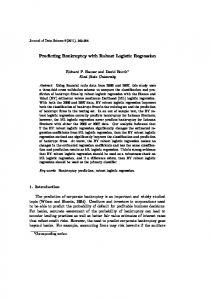
The following table compares the results of the different procedures for the infection data set. We concentrate on the estimate of the odds ratio for treatment with its 95% Wald confidence interval (which in some cases can be estimated within the procedures and in other cases requires an additional small calculation by hand or in an additional data step): Method
OR
[95%-CI]
PROC FREQ PROC GENMOD %GLIMMIX (B/C) %GLIMMIX (W/O’C) %NLINMIX (Method 1) %NLINMIX (Method 2) %NLINMIX (Method 3) PROC NLMIXED PROC PHREG PROC LOGISTIC FE-Meta-Analysis RE-Meta-Analysis
1.498 1.740 2.063 2.069 1.728 2.021 1.737 2.093 2.130 2.130 1.950 1.950
[0.915; 2.452] [1.102; 2.747] [1.154; 3.688] [1.176; 3.641] [1.109; 2.693] [1.076; 3.794] [1.112; 2.714] [1.162; 3.771] [1.177; 3.855] [1.137; 4.079] [1.057; 3.595] [1.057; 3.595]
Other brand and product names are registered trademarks or trademarks of their respective companies.
REFERENCES Allison, P.D. (1999), Logistic Regression Using the SAS System: Theory and Application, Cary, NC, SAS Institute Inc. Beitler, P.J., Landis, J.R. (1985), “A Mixed-effects Model for Categorical Data,“ Biometrics, 41, 991-1000. Breslow, N.R., Day, N.E. (1980), Statistical Methods in Cancer Research, Vol. II: The Design and Analysis of Cohort Studies, IARC, Lyon. Breslow, N.R., Clayton, D.G. (1993), “Approximate inference in generalized linear mixed models,“ Journal of the American Statistical Association, 88, 9-25. Brown, H., Prescott, R. (1999), Applied Mixed Models in Medicine, John Wiley & Sons, Chichester. Davidian, M. (2001), Nonlinear Models for Univariate and Multivariate Response, Lecture Notes, http://www.stat.ncsu.edu/~st762_info/davidian/notes/chap14.ps Derr, R.E. (2000), “Performing Exact Logistic Regression with the th SAS System,“ Proceedings of the 25 Annual SASâ Users Group International Conference (SUGI 25), 254-25. Diggle, P.J., Liang, K.-Y., Zeger, S.L. (1994), Analysis of Longitudinal Data, Oxford University Press, Oxford. Liang, K.-Y., Zeger, S.L. (1986), Longitudinal Data Analysis Using Generalized Linear Models, Biometrika, 73, 13-22. Littell, R.C., Milliken G.A., Stroup W.W., Wolfinger, R.D. (1996), SAS System for Mixed Models, Cary, NC, SAS Institute Inc. McCullagh, P., Nelder J.A. (1989), Generalized Linear Models, Chapman and Hall, New York. Normand, S.L. (1999), “Tutorial in Biostatistics. Meta-analysis: formulating, evaluating, combining and reporting,” Statistics in Medicine, 18, 321-359. Stijnen, T. (2000), “Letter to the editor,” Statistics in Medicine, 19, 759-761. Wolfinger, R.D., O’Connell, M. (1993), “Generalized linear models: a pseudo-likelihood approch,” Journal of Statistical Computation and Simulation, 48, 233-243. Wolfinger, R.D. (1997), “Comment: Experiences with the SAS Macro NLINMIX,” Statistics in Medicine, 16, 1258-1259. Wolfinger, R.D., Lin, X. (1997), “Two Taylor-series approximation methods for nonlinear mixed models,” Computational Statistics & Data Analysis, 25, 465-490. Wolfinger, R.D. (1999), “Fitting Nonlinear Mixed Models with the th new NLMIXED Procedure,” Proceedings of the 24 Annual SASâ Users Group International Conference (SUGI 24), 287-24. Zeger, S.L., Liang, K.Y., Albert, P.S. (1988), “Models for Longitudinal Data: A Generalized Estimating Equation Approach,” Biometrics, 77, 642-648
Calculating the crude odds ratio ignoring the clinic effect completely (FREQ procedure) underestimates the treatment effect grossly and even fails to reach statistical significance. All of the methods that calculate the marginal odds ratio (GENMOD procedure, %NLINMIX (Method 3)) result in smaller estimates for the treatment effect compared to the odds ratios from the random effects model. It can be shown that this is necessarily the case and one can even calculate a multiplicative factor that converts the estimates from the marginal to the random effect model (Zeger, Liang, Albert, 1988). Allison, 1999, explains this phenomenon in more detail and calls it “heterogeneity shrinkage” because the difference between marginal and random effects grows with increasing heterogeneity between clinics. The methods that estimate the random effects model deliver very similar estimates of the treatment effect (with the exception of %NLINMIX (Method 1)) and declare the odds ratio for treament a little bigger than 2, that is, the chance for curing the infection is more than doubled in the treatment group. Note that the estimates from the conditional ML method (PHREG/LOGISTIC procedure) are identical and that proceeding to the exact method merely enlarges the confidence interval by a small amount. The Meta-Analysis estimates from the fixed and the random effects model are identical. That means that the random effect model considers the between-clinic heterogeneity as statistically nonsignificant and automatically sets it to zero. This is in some contradiction to the estimated ν2 (not shown) from the other methods.
CONCLUSION The SAS System offers a large number of options for estimating logistic regression models with correlated data. It is difficult to give definite general recommendations which of the methods to use because this depends on the data at hand and on the desired interpretation of parameters (population-averaged vs. subjectspecific). For our infection data set we feel most comfortable with the results from the NLMIXED procedure and from the conditional ML analysis because (1) the heterogeneity between clinics is explicitly modelled and not considered as a nuisance effect, (2) they give exact ML estimates compared to the approximate ML estimates from %GLIMMIX and %NLINMIX, and (3) they are nearly identical under the differing assumptions of a normal distributed random effect (NLMIXED) and a complete removal of the random effect from the likelihood function.
CONTACT INFORMATION Oliver Kuss Institute of Medical Epidemiology, Biostatistics, and Informatics, Medical Faculty, University of Halle-Wittenberg 06097 Halle/Saale, Germany Phone: +49-345-5573582 Fax: +49-345-5573580 Email:
[email protected] WWW: http://imebmi.medizin.uni-halle.de/
5