HTL Perturbation Theory to Two Loops

hep-ph/0205085 DUKE-TH-02-221 ITF-UU-02/24 February 1, 2008

arXiv:hep-ph/0205085v1 9 May 2002

HTL Perturbation Theory to Two Loops Jens O. Andersen Institute for Theoretical Physics, University of Utrecht, Leuvenlaan 4, 3584 CC Utrecht, The Netherlands

Eric Braaten and Emmanuel Petitgirard Physics Department, Ohio State University, Columbus OH 43210, USA

Michael Strickland Physics Department, Duke University, Durham NC 27708, USA

Abstract We calculate the pressure for pure-glue QCD at high temperature to two-loop order using hard-thermal-loop (HTL) perturbation theory. At this order, all the ultraviolet divergences can be absorbed into renormalizations of the vacuum energy density and the HTL mass parameter. We determine the HTL mass parameter by a variational prescription. The resulting predictions for the pressure fail to agree with results from lattice gauge theory at temperatures for which they are available.

1

I. INTRODUCTION

Relativistic heavy-ion collisions allow the experimental study of hadronic matter at energy densities exceeding that required to create a quark-gluon plasma. A quantitative understanding of the properties of a quark-gluon plasma is essential in order to determine whether it has been created. Because QCD is asymptotically free, its running coupling constant αs becomes weaker as the temperature increases. One might therefore expect the behavior of hadronic matter at sufficiently high temperature to be calculable using perturbative methods. Unfortunately, a straightforward perturbative expansion in powers of αs does not seem to be of any quantitative use even at temperatures orders of magnitude higher than those achievable in heavy-ion collisions. The problem is evident in the free energy F of the quark-gluon plasma, whose weakcoupling expansion has been calculated through order αs5/2 [1–3]. For a pure-glue plasma, the first few terms in the weak-coupling expansion are FQCD

"

15 αs αs 3/2 = Fideal 1 − + 30 4 π π    2 αs 11 µ αs 135 log − log + 3.51 + 2 π 36 2πT π #    5/2 495 µ αs 3 + log − 3.23 + O(αs log αs ) , 2 2πT π 



(1)

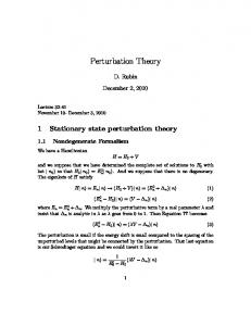
where Fideal = −(8π 2 /45)T 4 is the free energy of an ideal gas of massless gluons and αs = αs (µ) is the running coupling constant in the MS scheme. In Fig. 1, the free energy is shown as a function of the temperature T /Tc , where Tc is the critical temperature for the deconfinement transition. The weak-coupling expansions through orders αs , αs3/2 , αs2 , and αs5/2 are shown as bands that correspond to varying the renormalization scale µ by a factor of two from the central value µ = 2πT . As successive terms in the weak-coupling expansion are added, the predictions change wildly and the sensitivity to the renormalization scale grows. It is clear that a reorganization of the perturbation series is essential if perturbative calculations are to be of any quantitative use at temperatures accessible in heavy-ion collisions. The free energy can also be calculated nonperturbatively using lattice gauge theory [4]. The thermodynamic functions for pure-glue QCD have been calculated with high precision by Boyd et al. [5]. There have also been calculations with Nf = 2 and 4 flavors of dynamical quarks [6]. In Fig. 1, the lattice results for the free energy of pure-glue QCD from Boyd et al. [5] are shown as diamonds. The free energy is very close to zero near Tc . As the temperature increases, the free energy increases and approaches that of an ideal gas of massless gluons. We will regard the lattice results as the correct results for the thermodynamic functions. One goal of any reorganization of perturbation theory is to obtain a free energy that agrees within its domain of validity with the lattice results. There is of course little to be gained by just reproducing the results of lattice gauge theory. A method for reorganizing perturbation theory is of practical use only if it allows the calculation of quantities that are not so easily calculated using lattice gauge theory. There are many observables that are difficult or even impossible to calculate using lattice gauge 2

FIG. 1. The free energy for pure-glue QCD as a function of T /Tc . The weak-coupling expan3/2 5/2 sions through orders αs , αs , α2s , and αs are shown as bands that correspond to varying the renormalization scale µ by a factor of two. The diamonds are the lattice result from Boyd et al. [5]. The size of the diamonds indicate the typical error bar.

theory. First, lattice gauge theory becomes increasingly inefficient at higher temperatures, so some other method is required to extrapolate to high T . Second, calculations with light dynamical quarks require orders of magnitude more computer power than pure-glue QCD. Third, the Monte Carlo approach used in lattice gauge theory fails completely at nonzero baryon number density. Finally, lattice gauge theory is only effective for calculating static quantities, but many of the more promising signatures for a quark-gluon plasma involve dynamical quantities. The only rigorous method available for reorganizing perturbation theory in thermal QCD is dimensional reduction to an effective 3-dimensional field theory [7,8]. The coefficients of the terms in the effective lagrangian are calculated using perturbation theory, but calculations within the effective field theory are carried out nonperturbatively using lattice gauge theory. Dimensional reduction has the same limitations as ordinary lattice gauge theory: it can be applied only to static quantities and only at zero baryon number density. Unlike in ordinary lattice gauge theory, light dynamical quarks do not require any additional computer power, because they only enter through the perturbatively calculated coefficients in the effective lagrangian. This method has been applied to the Debye screening mass for QCD [8] as well as the pressure [7]. There are some proposals for reorganizing perturbation theory in QCD that are essentially just mathematical manipulations of the weak coupling expansion. The methods include Pad´e approximates [9], Borel resummation [10], and self-similar approximates [11]. These methods are used to construct more stable sequences of successive approximations 3

that agree with the weak-coupling expansion when expanded in powers of αs . These methods can only be applied to quantities for which several orders in the weak-coupling expansion are known, so they are limited in practice to the thermodynamic functions. One promising approach for reorganizing perturbation theory in thermal QCD is to use a variational framework. The free energy F is expressed as the variational minimum of a thermodynamic potential Ω(T, αs ; m2 ) that depends on one or more variational parameters that we denote collectively by m2 : 2

F (T, αs ) = Ω(T, αs ; m

)

.

(2)

∂Ω/∂m2 =0

A particularly compelling variational formulation is the Φ-derivable approximation, in which the complete propagator is used as an infinite set of variational parameters [12]. The Φderivable thermodynamic potential Ω is the 2PI effective action, the sum of all diagrams that are 2-particle-irreducible with respect to the complete propagator [13]. The n-loop Φ-derivable approximations, in which Ω is the the sum of 2PI diagrams with up to n loops, form a systematically improvable sequence of variational approximations. Until recently, Φderivable approximations have proved to be intractable for relativistic field theories except for simple cases in which the self-energy is momentum-independent. However there has been some recent progress in solving the 3-loop Φ-derivable approximation for scalar field theories. Braaten and Petitgirard have developed an analytic method for solving the 3loop Φ-derivable approximation for the massless φ4 field theory [14]. Van Hees and Knoll have developed numerical methods for solving the 3-loop Φ-derivable approximation for the massive φ4 field theory [15]. They have also investigated renormalization issues associated with the Φ-derivable approximation. The application of the Φ-derivable approximation to QCD was first discussed by McLerran and Freedman [16]. One problem with this approach is that the thermodynamic potential Ω is gauge dependent, and so are the resulting thermodynamic functions. The gauge dependence is the same order in αs as the truncation error. However the most serious problem is that even the 2-loop Φ-derivable approximation has proved to be intractable. The 2-loop Φ-derivable approximation for QCD has been used as the starting point for HTL resummations of the entropy by Blaizot, Iancu and Rebhan [17] and of the pressure by Peshier [18]. The thermodynamic potential Ω2−loop is a functional of the complete gluon propagator Dµν (P ). The HTL resummations of Refs. [17] and [18] can be derived in 2 steps. The first step is to replace the 2-loop functional at its variational point by a 1-loop functional evaluated at the 2-loop variational point. In the resummation of the pressure of Ref. [18], the 2-loop functional is the thermodynamic potential and this step is a weakcoupling approximation: Ω2−loop [Dµν ]

δΩ2−loop =0

≈

Ω1−loop [Dµν ]

.

(3)

δΩ2−loop =0

In the resummation of the entropy of Ref. [17], the 2-loop functional is the derivative of Ω2−loop with respect to T and this step is an exact equality. The second step exploits the HTL fact that the HTL gluon propagator Dµν (P ) is an approximate solution to the variational equation δΩ2−loop = 0. The HTL gluon propagator depends on one parameter m2D , which 4

can be interpreted as the Debye screening mass for the gluon. The HTL gluon propagator satisfies the variational equation to leading order in αs provided that m2D reduces in the weak-coupling limit to m2D =

4πNc αs (µ)T 2 , 3

(4)

with some appropriate choice for the scale µ such as µ = 2πT . Thus we can approximation HTL the solution to the variational equation in (3) by Dµν (P ): Ω1−loop [Dµν ]

δΩ2−loop =0

≈



HTL Ω1−loop [Dµν ]

m2D =4παs T 2

.

(5)

This approximate solution holds when m2D is given by (4), however, there is some freedom in the choice of the parameter m2D , as long as it reduces to (4) in the weak-coupling limit. It can not be determined variationally, because the variational character of the thermodynamic potential was lost in the first step (3). With the prescription (4), the errors in the thermodynamic functions are of order αs3/2 . The errors can be reduced to order αs2 by adding an αs3/2 term to the right side of (4). The intractability of Φ-derivable approximations motivates the use of simpler variational approximations. One such strategy that involves a single variational parameter m has been called optimized perturbation theory [19], variational perturbation theory [20], or the linear δ expansion [21]. This strategy was applied to the thermodynamics of the massless φ4 field theory by Karsch, Patkos and Petreczky under the name screened perturbation theory [22]. The method has also been applied to spontaneously broken field theories at finite temperature [23]. The calculations of the thermodynamics of the massless φ4 field theory using screened perturbation theory have been extended to 3 loops [24]. The calculations can be greatly simplified by using a double expansion in powers of the coupling constant and m/T [25]. HTL perturbation theory (HTLpt) is an adaptation of this strategy to thermal QCD [26]. The exactly solvable theory used as the starting point is one whose propagators are the HTL gluon propagators. The variational mass parameter mD can be identified with the Debye screening mass. The one-loop free energy in HTLpt was calculated for pure-glue QCD in Ref. [26] and for QCD with light quarks in Ref. [27]. At this order, the parameter mD cannot be determined variationally, so the prescription (4) was used. The resulting thermodynamic functions have errors of order αs , but the terms of order αs3/2 associated with Debye screening are correct. A two-loop calculation is required to reduce the errors to order αs2 . At two-loop order, it is also possible to determine mD using a variational prescription. One difference between HTLpt and the HTL resummation methods of Refs. [17] and [18] is in how they deal with gauge invariance. HTLpt is constructed in such a way that physical observables are gauge invariant order-by-order in perturbation theory. Gauge invariance arises in the same way as in ordinary perturbation theory by cancellations between diagrams. In the HTL resummation methods of Refs. [17] and [18], the 2-loop thermodynamic potential Ω2−loop that is used as the starting point is gauge dependent. In the first step (3) of the derivation, Ω2−loop is replaced by a 1-loop functional Ω1−loop that is gauge invariant, but the variational equation δΩ2−loop = 0 is still gauge dependent. In the second step (5), the 5

HTL solution to that variational equation is approximated by Dµν , and it is only at this point that the gauge dependence disappears. Another difference between HTLpt and the HTL resummation methods of Refs. [17] and [18] is in the ranges of observables to which they can be applied. The HTL resummation methods were specifically formulated as approximations to the thermodynamic functions, so they cannot be easily applied to other observables. However, they can be used to calculate the thermodynamic functions in cases where calculations using conventional lattice gauge theory are difficult or impossible: the high-temperature limit of pure-glue QCD, QCD with light quarks, and QCD with nonzero baryon number density. In contrast to these methods, HTLpt has the same wide range of applicability as ordinary perturbation theory. It can be used to calculate the thermodynamic functions, but it can also be applied to all the standard signatures of a quark-gluon plasma. It has some of the limitations of ordinary perturbation theory. Calculations can be carried out only up to the order at which the magnetic screening problem causes diagrammatic methods to break down. In this paper, we calculate the thermodynamic functions of QCD to 2-loop order in HTLpt. We begin with a brief summary of HTLpt in Section II. In Section III, we give the expressions for the one-loop and two-loop diagrams for the thermodynamic potential. In Section IV, we reduce those diagrams to scalar sum-integrals. We are unable to compute those sum-integrals, so in Section V, we evaluate them approximately by expanding them in powers of mD /T . The diagrams are combined in Section VI to obtain the final results for the two-loop thermodynamic potential up to 5th order in g and mD /T . In Section VII, we present our numerical results for the thermodynamic functions of QCD. There are several appendices that contain technical details of the calculations. In Appendix A, we give the Feynman rules for HTLpt in Minkowski space to facilitate the application of this formalism to signatures of the quark-gluon plasma. The most difficult aspect of these calculations was the evaluation of the sum-integrals obtained from the expansion in mD /T . We give the results for these sum-integrals in Appendix B. The evaluation of some difficult thermal integrals that were required to obtain the sum-integrals is described in Appendix C.

II. HTL PERTURBATION THEORY

The lagrangian density that generates the perturbative expansion for pure-glue QCD can be expressed in the form 1 LQCD = − Tr (Gµν Gµν ) + Lgf + Lghost + ∆LQCD , (6) 2 where Gµν = ∂µ Aν − ∂ν Aµ − ig[Aµ , Aν ] is the gluon field strength and Aµ is the gluon field expressed as a matrix in the SU(Nc ) algebra. The ghost term Lghost depends on the choice of the gauge-fixing term Lgf . Two choices for the gauge-fixing term that depend on an arbitrary gauge parameter ξ are the general covariant gauge and the general Coulomb gauge:  1  covariant , (7) Lgf = − Tr (∂ µ Aµ )2 ξ  1  Coulomb . (8) = − Tr (∇ · A)2 ξ 6

The perturbative expansion in powers of g generates ultraviolet divergences. The renormalizability of perturbative QCD guarantees that all divergences in physical quantities can be removed by renormalization of the coupling constant αs = g 2/4π. If we use dimensional regularization with minimal subtraction as a renormalization prescription, the renormalization can be accomplished by substituting αs → αs + ∆αs , where the counterterm ∆αs is a power series in αs whose coefficients have only poles in ǫ: 11Nc 2 17Nc2 121Nc2 ∆αs = − αs3 + O(αs4) . αs + − 12πǫ 144π 2 ǫ2 48π 2 ǫ !

(9)

Renormalized perturbation theory can be implemented by including among the interactions terms a counterterm lagrangian ∆LQCD that is given by the change in the first 3 terms on the right side of (6) upon substituting g → g(1 + ∆αs )1/2 . Hard-thermal-loop perturbation theory (HTLpt) is a reorganization of the perturbation series for thermal QCD. The lagrangian density is written as

L = (LQCD + LHTL)

The HTL improvement term is

√ g→ δg



*

+ ∆LHTL .

α β

y y 1 LHTL = − (1 − δ)m2D Tr Gµα 2 (y · D)2

+

y

(10)



Gµβ  ,

(11)

ˆ ) is a light-like where Dµ is the covariant derivative in the adjoint representation, y µ = (1, y ˆ . The term (11) has the four-vector, and h. . .iy represents the average over the directions of y form of the effective lagrangian that would be induced by a rotationally invariant ensemble of colored sources with infinitely high momentum. The parameter mD can be identified with the Debye screening mass. HTLpt is defined by treating δ as a formal expansion parameter. The free lagrangian in general covariant gauge is obtained by setting δ = 0 in (10):  1  Lfree = −Tr (∂µ Aν ∂ µ Aν − ∂µ Aν ∂ ν Aµ ) − Tr (∂ µ Aµ )2 ξ 

1 y αy β − m2D Tr (∂µ Aα − ∂α Aµ ) 2 (y · ∂)2 *

+

y



(∂ µ Aβ − ∂β Aµ ) .

(12)

The resulting propagator is the HTL gluon propagator. The remaining terms in (10) are treated as perturbations. The Feynman rules for gluon and ghost propagators and the 3-gluon, ghost-gluon, and 4-gluon vertices are given in Appendix A. The HTL perturbation expansion generates ultraviolet divergences. In QCD perturbation theory, renormalizability constrains the ultraviolet divergences to have a form that can be cancelled by the counterterm lagrangian ∆LQCD . There is no proof that the HTL perturbation expansion is renormalizable, so the general structure of the ultraviolet divergences is not known. The most optimistic possibility is that HTLpt is renormalizable, so that the ultraviolet divergences in physical quantities can all be cancelled by renormalization of the coupling constant αs , the mass parameter m2D , and the vacuum energy density E0 . If this 7

is the case, the renormalization of a physical quantity can be accomplished by substituting αs → αs + ∆αs and m2D → m2D + ∆m2D , where ∆αs and ∆m2D are counterterms. In the case of the free energy, it is also necessary to add a vacuum energy counterterm ∆E0 . If we use dimensional regularization with minimal subtraction as a renormalization prescription, the form of the counterterms for δαs , (1 − δ)m2D , and E0 should be the power of (1 − δ)m2D required by dimensional analysis multiplied by a power series in δαs with coefficients that have only poles in ǫ. The counterterm for δαs should be identical to that in ordinary perturbative QCD given in (9) with: 17Nc2 3 3 121Nc2 11Nc 2 2 δ αs + O(αs4 ) . δ αs + − δ∆αs = − 12πǫ 144π 2 ǫ2 48π 2 ǫ !

(13)

The leading term in the delta expansion of the E0 counterterm ∆E0 was deduced in Ref. [26] by calculating the free energy to leading order in δ. The E0 counterterm ∆E0 must therefore have the form Nc2 − 1 + O(δαs ) (1 − δ)2 m4D . 2 128π ǫ !

∆E0 =

(14)

To calculate the free energy to next-to-leading order in δ, we need the counterterm ∆E0 to order δ and the counterterm ∆m2D to order δ. We will show that there is a nontrivial cancellation of the ultraviolet divergences if the mass counterterm has the form ∆m2D

=

11Nc δαs + O(δ 2 αs2 ) (1 − δ)m2D . − 12πǫ 



(15)

Renormalized perturbation theory can be implemented by including a counterterm lagrangian ∆LHTL among the interaction terms in (10). Physical observables are calculated in HTLpt by expanding them in powers of δ, truncating at some specified order, and then setting δ = 1. This defines a reorganization of the perturbation series in which the effects of the m2D term in (12) are included to all orders but then systematically subtracted out at higher orders in perturbation theory by the δm2D term in (11). If we set δ = 1, the lagrangian (10) reduces to the QCD lagrangian (6). If the expansion in δ could be calculated to all orders, all dependence on mD should disappear when we set δ = 1. However, any truncation of the expansion in δ produces results that depend on mD . Some prescription is required to determine mD as a function of T and αs . We choose to treat mD as a variational parameter that should be determined by minimizing the free energy. If we denote the free energy truncated at some order in δ by Ω(T, αs , mD , δ), our prescription is ∂ Ω(T, αs , mD , δ = 1) = 0. ∂mD

(16)

Since Ω(T, αs , mD , δ = 1) is a function of a variational parameter mD , we will refer to it as the thermodynamic potential. We will refer to the variational equation (16) as the gap equation. The free energy F is obtained by evaluating the thermodynamic potential at the solution to the gap equation. Other thermodynamic functions can then be obtained by taking appropriate derivatives of F with respect to T . 8

III. DIAGRAMS FOR THE THERMODYNAMIC POTENTIAL

The thermodynamic potential at leading order in HTL perturbation theory (HTLpt) is ΩLO = (Nc2 − 1)Fg + ∆0 E0 ,

(17)

where Fg is the contribution to the free energy from each of the color states of the gluon: Fg = −

1P {(d − 1) log[−∆T (P )] + log ∆L (P )} . 2 P Z

(18)

The transverse and longitudinal HTL propagators ∆T (P ) and ∆L (P ) are given in (A.49) and (A.50). We use dimensional regularization with d = 3 − 2ǫ spatial dimensions to regularize ultraviolet divergences. The term of order δ 0 in the vacuum energy counterterm was determined in Ref. [26]: ∆0 E0 =

Nc2 − 1 4 m . 128π 2 ǫ D

(19)

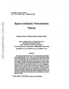
FIG. 2. Diagrams contributing through NLO in HTLpt. Shaded circles indicate dressed HTL propagators and vertices.

The thermodynamic potential at next-to-leading order in HTLpt can be written ΩNLO = ΩLO + (Nc2 − 1) [F3g + F4g + Fgh + FHTL ] + ∆1 E0 + ∆1 m2D

∂ ΩLO , ∂m2D

(20)

where ∆1 E0 and ∆1 m2D are the terms of order δ in the vacuum energy density and mass counterterms. The contributions from the two-loop diagrams with the three-gluon and fourgluon vertices are Z Nc 2 P g Γµλρ (P, Q, R)Γνστ (P, Q, R)∆µν (P )∆λσ (Q)∆ρτ (R) , 12 PQ Z Nc 2 P g Γµν,λσ (P, −P, Q, −Q)∆µν (P )∆λσ (Q) . = 8 PQ

F3g =

(21)

F4g

(22)

Expressions for the gluon propagator tensor ∆µν , the 3-gluon vertex tensor Γµλρ , and the 4-gluon vertex tensor Γµν,λσ in Minkowski space are given in (A.25) or (A.26), (A.32), and (A.41). Prescriptions for translating them into the Euclidean tensors appropriate for the imaginary time formalism are given in Appendix A 7. The contribution from the ghost 9

diagram depends on the choice of gauge. The expressions in the covariant and Coulomb gauges are Fgh

Z Nc 2 P = g 2 PQ Z Nc 2 P = g 2 PQ

1 1 µ ν µν Q R ∆ (P ) Q2 R2 1 1 (Qµ − Q·n nµ ) (Rν − R·n nν ) ∆µν (P ) 2 2 q r

covariant ,

(23)

Coulomb .

(24)

The contribution from the HTL counterterm diagram is FHTL

1 P µν Π (P )∆µν (P ) . = 2 P Z

(25)

It can also be obtained by substituting m2D → (1 − δ)m2D in the one-loop expression Fg in (18) and expanding to first order in δ: FHTL =

1P [(d − 1)ΠT (P )∆T (P ) − ΠL (P )∆L (P )] . 2 P Z

(26)

Provided that HTLpt is renormalizable, the ultraviolet divergences at any order in δ can be cancelled by renormalizations of the vacuum energy density E0 , the HTL mass parameter m2D , and the coupling constant αs . Renormalization of the coupling constant does not enter until order δ 2 . We will calculate the thermodynamic potential as a double expansion in powers of g and mD /T , including all terms through 5th order. The δαs term in ∆E0 does not contribute until 6th order in this expansion, so the term of order δ in ∆E0 can be obtained simply by expanding (19) to first order in δ: ∆1 E0 = −

Nc2 − 1 4 m . 64π 2 ǫ D

(27)

The remaining ultraviolet divergences must be removed by renormalization of the mass parameter mD . We will find that there are ultraviolet divergences in the αs m2D T 2 and αs m3D T 3 terms, and both are removed by the same counterterm ∆1 m2D . This provides nontrivial evidence for the renormalizability of HTLpt at this order in δ. The sum of the 3-gluon, 4-gluon, and ghost contributions in (21), (22), and (23) or (24) is gauge-invariant. By inserting the expression (A.25) or (A.26) for the gluon propagator tensor and using the Ward identities (A.35) and (A.42), one can easily verify that the sum of these three diagrams is independent of the gauge parameter ξ in both covariant gauge and Coulomb gauge. With more effort, we can verify the equivalence of the covariant gauge expression with ξ = 0 (Landau gauge) and the Coulomb gauge expression with ξ = 0. This involves expanding the tensor nµP nνP in the covariant gauge propagator into the sum of terms proportional to nµ nν , P µ nν , nµ P ν , and P µ P ν , and then applying the Ward identities to the terms involving P µ or P ν . IV. REDUCTION TO SCALAR SUM-INTEGRALS

The first step in calculating the thermodynamic potential is to reduce the sum of the diagrams to scalar sum-integrals. The one-loop diagram in (18) and the HTL counterterm 10

diagram (25) are already expressed in terms of scalar integrals. We proceed to consider the 3-gluon diagram in (21), the 4-gluon diagram in (22), and the ghost diagram in Landau gauge which is given in (23). The expression for the sum of these three diagrams is simpler than that of the 3-gluon diagram alone. We insert the gluon propagator in the form (A.29) with ξ = 0. It has terms proportional to ∆T and ∆X , where ∆X is the combination of transverse and longitudinal propagators defined in (A.27). When a momentum P µ from the gluon propagator tensor is contracted with a 3-gluon or 4-gluon vertex, the Ward identities can be used to reduce it ultimately to expressions involving the inverse propagator (A.20). The term ∆T /∆L can be eliminated in favor of ∆X /∆L using the definition (A.27). This reduces the sum of the 3-gluon, 4-gluon, and ghost diagrams to the following form: F3g + F4g + Fgh ( Z Nc 2P = g Γµνλ Γµνλ ∆T (P )∆T (Q)∆T (R) − 3Γµν0 Γµν0 ∆T (P )∆T (Q)∆X (R) 12 PQ 

+3Γµ00 Γµ00 ∆T (P )∆X (Q)∆X (R) − Γ000

2

∆X (P )∆X (Q)∆X (R) 3 +3d(d + 1) ∆T (P )∆T (Q) − 6d ∆T (P )∆X (Q) + Γ00,00 ∆X (P )∆X (Q) 2 ! Q·R n·Q n·R +6 ∆T (P ) − ∆X (P ) 2 2 QR Q2 R2 ! n·Q n·R ∆X (Q) n·Q nQ ·R ∆T (P ) − ∆X (P ) −12 2 2 2 2 q R QR ∆L (Q) ) ! n·Q n·R nQ ·nR n·Q n·R ∆X (Q) ∆X (R) +6 . (28) ∆T (P ) − ∆X (P ) q2 r2 Q2 R2 ∆L (Q) ∆L (R)

In the 3-gluon and 4-gluon vertex tensors, we have suppressed the momentum arguments: Γµνλ = Γµνλ (P, Q, R) and Γ00,00 = Γ00,00 (P, −P, Q, −Q). The next step is to insert the Euclidean analogs of the expressions (A.32) and (A.41) for the 3-gluon and 4-gluon vertex tensors. The combinations of terms that appear in (28) can be simplified using the “Ward identities” (A.3), (A.34), and (A.38) satisfied by the HTL correction tensors: Γµνλ Γµνλ = 3d(P 2 + Q2 + R2 ) + m4D T µνλ T µνλ , Γµν0 Γµν0 = p2 + q 2 + 4r 2 + 2d(n·P )2 + 2d(n·Q)2 − d(n·R)2 +2m2D (2TR − TP − TQ ) + m4D T µν0 T µν0 , 2 Γµ00 Γµ00 = 2q 2 + 2r − p2 i h −2m2D 2TP − TQ − TR + n·(Q − R) T 000 + m4D T µ00 T µ00 , 000 2

m4D

000 2

(Γ ) = (T ) , 00,00 2 Γ = −mD T 0000 .

(29) (30) (31) (32) (33)

In the 3-gluon and 4-gluon HTL correction tensors, we have suppressed the momentum arguments: T µνλ = T µνλ (P, Q, R) and T 0000 = T 0000 (P, Q, −P, −Q). We have also used the short-hand TP = −T 00 (P, −P ) for the 2-gluon HTL correction tensor. Inserting the expressions (29)–(33) into (28) and eliminating 1/∆L (P ) in favor of TP , the reduction to scalar integrals is 11

F3g + F4g + Fgh (  Z Nc 2 P 1 = 3dR2 + m4D T µνλ T µνλ ∆T (P )∆T (Q)∆T (R) g 4 3 PQ h

+ −2q 2 − 4r 2 − 4d(n·Q)2 + d(n·R)2 h

i

−4m2D (TR − TQ ) − m4D T µν0 T µν0 ∆T (P )∆T (Q)∆X (R)

+ −p2 + 4r 2 − 2m2D n·(Q − R) T 000

i

−4m2D (TP − TR ) + m4D T µ00 T µ00 ∆T (P )∆X (Q)∆X (R)

1 − m4D (T 000 )2 ∆X (P )∆X (Q)∆X (R) 3 +d(d + 1) ∆T (P )∆T (Q) − 2d ∆T (P )∆X (Q) 1 − m2D T 0000 ∆X (P )∆X (Q) 2   Q·R +2 2 2 ∆T (P ) 1 − [q 2 + m2D (1 − TQ )]∆X (Q) QR 







× 1 − [r 2 + m2D (1 − TR )]∆X (R)

−2

  n·Q n·R 2 2 ∆ (P ) 1 − [q + m (1 − T )]∆ (Q) X Q X D Q2 R2

× 1 − [r 2 + m2D (1 − TR )]∆X (R)

q·r 2 [q + m2D (1 − TQ )] ∆T (P )∆X (Q) q 2 R2 (2n2Q − 1)q · r 2 [q + m2D (1 − TQ )][r 2 + m2D (1 − TR )] −2 q2 r2 +4

)

×∆T (P )∆X (Q)∆X (R) .

(34)

V. EXPANSION IN THE MASS PARAMETER

The thermodynamic potential has been reduced to scalar sum-integrals. In Ref. [26], the sum-integrals for the one-loop free energy were evaluated exactly by replacing the sums by contour integrals, extracting the poles in ǫ, and then reducing the momentum integrals to integrals that were at most two-dimensional and could therefore be easily evaluated numerically. It was also shown that the sum-integrals could be expanded in powers of mD /T , and that the first few terms in the expansion gave a surprisingly accurate approximation to the exact result. If we tried to evaluate the 2-loop HTL free energy exactly, there are terms such as those involving T µνλ T µνλ that could at best be reduced to 5-dimensional integrals that would have to be evaluated numerically. We will therefore evaluate the sum-integrals approximately by expanding them in powers of mD /T . We will carry out the mD /T expansion to high enough order to include all terms through order g 5 if mD /T is taken to be of order g. 12

A. 1-loop sum-integrals

The one-loop sum-integrals include the leading order free energy given by the sumintegrals (18) and the HTL counterterm given by (26). The leading order free energy must be expanded to order (mD /T )5 in order to include all terms through order g 5 . The HTL counterterm has an explicit factor of m2D , so the sum-integral for the HTL counterterm diagram need only to be expanded to order (mD /T )3 to include all terms through order g 5. The sum-integrals over P involve two momentum scales: mD and T . In order to expand them in powers of mD /T , we separate them into contributions from hard loop momentum, for which some of the components of P are of order T , and soft loop momenta, for which all the components of P are of order mD . We will denote these regions by (h) and (s). Since the Euclidean energy P0 is an integer multiple of 2πT , the soft region requires P0 = 0. 1. Hard contributions

If P is hard, the denominators P 2 + ΠT and p2 + ΠL in the propagators are of order T , but the self-energy functions ΠT and ΠL are of order m2D . The mD /T expansion can therefore be obtained by expanding in powers of ΠT and ΠL . For one-loop free energy, we need to expand to second order in m2D : Fg(h) =

d − 1P 1 P 1 log(P 2 ) + m2D 2 P 2 P P2 # Z " 1 1 1 1 1 1 4 P 2 m − 2 2 2 − 2d 4 TP + 2 2 2 TP + d 4 (TP ) . − 4(d − 1) D P (P 2 )2 p P p pP p Z

Z

(35)

Note that the function TP cancels from the m2D term because of the identity (A.12). The values of the sum-integrals are given in Appendix B. Inserting those expressions, the hard contributions to the leading-order free energy reduce to Fg(h)

π2 = − T4 + 45 1 − 128π 2

"

! #

ζ ′(−1) µ 2ǫ 2 2 1 1+ 2+2 ǫ mD T 24 ζ(−1) 4πT !  µ 2ǫ 4 2π 2 1 − 7 + 2γ + mD . ǫ 3 4πT 

(36)

Note that the pole in the m4D term is cancelled by the counterterm (19). The HTL counterterm diagram has an explicit factor of m2D , so we need only to expand the sum-integral to first order in m2D . Eliminating ΠT (P ) and ΠL (P ) in favor of the function TP , the result is 1 P 1 (h) Fct = − m2D 2 P P2 # Z " 1 1 1 1 1 1 P + m4 − 2 2 2 − 2d 4 TP + 2 2 2 TP + d 4 (TP )2 . 2(d − 1) D P (P 2 )2 p P p p P p Z

(37)

The values of the sum-integrals are given in Appendix B. Inserting those expressions, the hard contributions to the HTL counterterm in the free energy reduce to 13

(h) Fct

1 1 = − m2D T 2 + 24 64π 2

2π 2 1 − 7 + 2γ + ǫ 3

!

µ 4πT

2ǫ

m4D .

(38)

Note that the first term in (38) cancels the order-ǫ0 term in the coefficient of m2D T 2 in (36). We have kept the order-ǫ term in the coefficient of m2D T 2 in (36), because it will contribute to the final result through the mass counterterm. 2. Soft contributions

The soft contribution comes from the P0 = 0 term in the sum-integral. At soft momentum P = (0, p), the HTL self-energy functions reduce to ΠT (P ) = 0 and ΠL (P ) = m2D . The transverse term vanishes in dimensional regularization because there is no momentum scale in the integral over p. Thus the soft contribution comes from the longitudinal term only. The soft contribution to the leading order free energy is 1 Fg(s) = T 2

Z

p

log(p2 + m2D ) .

(39)

Using the expression for the integral in Appendix C, we obtain Fg(s)

8 1 1+ ǫ =− 12π 3 



µ 2mD

2ǫ

m3D T .

(40)

The soft contribution to the HTL counterterm is (s) Fct

1 = − m2D T 2

Z

p p2

1 . + m2D

(41)

Using the expression for the integral in Appendix C, we obtain (s)

Fct =

1 3 m T. 8π D

(42)

B. 2-loop sum-integrals

The sum of the two-loop sum-integrals is given in (34). Since these integrals have an explicit factor of g 2 , we need only expand the sum-integrals to order (mD /T )3 to include all terms through order g 5. The sum-integrals involve two momentum scales: mD and T . In order to expand them in powers of mD /T , we separate them into contributions from hard loop momenta and soft loop momenta. This gives 3 separate regions which we will denote (hh), (hs), and (ss). In the (hh) region, all 3 momenta P , Q, R are hard. In the (hs) region, two of the 3 momenta are hard and the other is soft. In the (ss) region, all 3 momenta are soft.

14

1. Contributions from (hh) region

If P , Q, R are all hard, we can obtain the mD /T expansion simply by expanding in powers of m2D . To obtain the expansion through order m3D /T 3 , we need only expand to first order in m2D , with ∆X and ΠT taken to be of order m2D : (hh) F3g+4g+gh

(

Nc 2P 3dR2 ∆T (P )∆T (Q)∆T (R) g = 4 PQ Z

i

h

+ −2q 2 − 4r 2 − 4d(n·Q)2 + d(n·R)2 ∆T (P )∆T (Q)∆X (R) +d(d + 1) ∆T (P )∆T (Q) − 2d ∆T (P )∆X (Q)   Q·R +2 2 2 ∆T (P ) 1 − 2q 2 ∆X (Q) QR ) q·r n·Q n·R ∆X (P ) + 4 2 ∆T (P )∆X (Q) . −2 Q2 R2 R

(43)

For hard momenta, the self-energies are suppressed by m2D /T 2 relative to the propagators, so they can be expanded in powers of ΠT and ΠL . Expanding all terms to first order in m2D , and using (A.6) and (A.7) to eliminate ΠT (P ) and ΠL (P ) in favor of TP , we obtain (hh) F3g+4g+gh

(

)

Nc 2 P 1 1 = (d − 1)2 2 2 g 4 P Q PQ ( Z Nc 2 2 P 1 1 1 1 + g mD + 2(d − 2) 2 2 2 − 2(d − 1) 2 2 2 4 P (Q ) P q Q PQ 1 1 +2 2 2 2 + (d + 2) 2 2 2 P QR P Qr q2 q2 P ·Q −2d 2 2 2 2 − 4d 2 2 2 2 + 4 2 2 2 2 P Q (r ) P Q (r ) P Qr R 1 1 1 −2(d − 1) 2 2 2 TQ − (d + 1) 2 2 2 TR P q Q P Qr ) 2 q P ·Q +4d 2 2 2 2 TR + 2d 2 2 2 2 TR . (44) P Q (r ) P Q (r ) Z

Inserting the sum-integrals from Appendix B, this reduces to (hh) F3g+4g+gh

7 1 Nc αs π 2 Nc αs 4 T − + 4.621 = 12 3π 96 ǫ 3π 





µ 4πT

4ǫ

m2D T 2 .

(45)

2. The (hs) contributions

In the (hs) region, the soft momentum can be any one of the three momenta P , Q, or R. However we can always permute the momenta so that the soft momentum is P = (0, p). The function that multiplies the soft propagator ∆T (0, p) or ∆X (0, p) can be expanded in powers of the soft momentum p. In the case of ∆T (0, p), the resulting integrals over p 15

have no scale and therefore vanish in dimensional regularization. The integration measure R 3 2 p scales like mD , the soft propagator ∆X (0, p) scales like 1/mD , and every power of p in the numerator scales like mD . The only terms that contribute through order g 2 m3D T are (hs)

F3g+4g+gh

Nc 2 = g T 4

Z

p

∆X (0, p)

Z ( P h

i

−2q 2 − 4p2 − 4d(n·Q)2 + 4m2D TQ ∆T (Q)∆T (R)

Q

i

h

+ 4r 2 − 2q 2 + 4p2 ∆T (Q)∆X (R)

 (n·Q)2  −2d∆T (Q) + 2 2 2 1 − 2q 2 ∆X (Q) QR

)

.

(46)

In the terms that are already of order g 2 m3D T , we can set R = −Q. In the terms of order g 2 mD T 3 , we must expand the sum-integrand to second order in p. After averaging over angles of p, the linear terms in p vanish and quadratic terms of the form pi pj are replaced by p2 δ ij /d. We can set p2 = −m2D , because any factor proportional to p2 + m2D will cancel the denominator of the integral over p, leaving an integral with no scale. Our expression for the (hs) contribution reduces to (hs) F3g+4g+gh

Z Nc 2 Z q2 1 1 P = g T + 2(d − 1) − (d − 1) 2 2 Q2 (Q2 )2 p p2 + mD Q ( Z Z 1 (d − 1)(d + 2) q 2 1 P + Nc g 2m2D T + − (d − 4) 2 (Q2 )2 d (Q2 )3 p p2 + mD Q ) 4(d − 1) q 4 . (47) − d (Q2 )4 )

(

Inserting the sum-integrals from Appendix B and the integrals from Appendix C, this reduces to π Nc αs (hs) F3g+4g+gh = − mD T 3 2 3π       µ 2ǫ µ 2ǫ 3 Nc αs 11 1 27 + + 2γ mD T . (48) − 32π ǫ 11 3π 4πT 2mD 3. The (ss) contributions

The (ss) contributions comes from the zero-frequency modes of the sum-integrals. The HTL correction functions TP , T 000 , and T 0000 vanish when all the external frequencies are zero. The self-energy functions at zero-frequency are ΠT (0, p) = 0 and ΠL (0, p) = m2D . The only scales in the integrals come from the longitudinal propagators ∆L (0, p) = 1/(p2 + m2D ). Therefore in dimensional regularization, at least one such propagator is required in order for the integral to be nonzero. The only terms in (34) that give nonzero contributions are (ss) F3g+4g+gh

Nc 2 2 = g T 4

Z

pq

(

h

h

i

−2q 2 − 4r 2 ∆T (0, p)∆T (0, q)∆X (0, r) 2

2

i

)

+ −p + 4r ∆T (0, p)∆X (0, q)∆X (0, r) . 16

(49)

After simplifying the integral by dropping terms that vanish in dimensional regularization, it reduces to (ss)

F3g+4g+gh =

Nc 2 2 g T 4

Z

pq

p2 + 4m2D . p2 (q 2 + m2D )(r 2 + m2D )

(50)

Inserting the integrals from Appendix C, this reduces to (ss) F3g+4g+gh

3 1 Nc αs = +3 16 ǫ 3π 





µ 2mD

4ǫ

m2D T 2 .

(51)

VI. THERMODYNAMIC POTENTIAL

In this section, we calculate the thermodynamic potential Ω(T, αs , mD , δ = 1) explicitly, first to leading order in the δ expansion and then to next-to-leading order. A. Leading order

The complete expression for the leading order thermodynamic potential is the sum of the contributions from 1-loop diagrams and the leading term (19) in the vacuum energy counterterm. The contributions from the 1-loop diagrams, including all terms through order g 5 , is the sum of (36) and (40): Ω1−loop = Fideal

(

45 15 2 ˆ D + 30m ˆ 3D + 1− m 2 8

1 µ ˆ 2π 2 m ˆ 4D + 2 log − 7 + 2γ + ǫ 2 3 !

)

,

(52)

where Fideal is the free energy of an ideal gas of Nc2 − 1 massless spin-one bosons, Fideal =

(Nc2

π2 − 1) − T 4 45

!

,

(53)

and m ˆ D and µ ˆ are dimensionless variables: mD , 2πT µ . µ ˆ= 2πT

m ˆD =

(54) (55)

Adding the counterterm (19), we obtain the thermodynamic potential at leading order in the delta expansion: ΩLO = Fideal

(

15 2 µ ˆ 7 45 π2 1− m log − + γ + m ˆ 4D ˆ D + 30m ˆ 3D + 2 4 2 2 3 !

)

.

(56)

The coefficient of m ˆ 4D in (56) differs from the result calculated previously in Ref. [26]. In that paper, the constant under the logarithm of µ ˆ/2 was − 23 +γ+log 2 instead of − 72 +γ+ 31 π 2 . 17

The reason for the difference is that the sum-integral Fg was calculated in Ref. [26] using dimensional regularization to regularize the integral, but using the 3-dimensional expressions for the HTL propagators ∆T and ∆L . At leading order, the difference can be absorbed into the definition of the scale µ. For calculations beyond leading order, it is essential for consistency to use the d-dimensional expressions for these propagators.1 B. Next-to-leading order

The complete expression for the next-to-leading order correction to the thermodynamic potential is the sum of the contributions from the 2-loop diagrams, the HTL counterterms, and renormalization counterterms. The contributions from the 2-loop diagrams, including all terms through order g 5 , is the sum of (45), (48), and (51): Ω2−loop = Fideal

Nc αs 3π

(

"

#

15 165 1 µ ˆ 72 − + 45 m ˆD − + 4 log − log m ˆ D + 1.969 m ˆ 2D 4 8 ǫ 2 11 " # ) µ ˆ 27 495 1 3 + 4 log − 2 log m ˆD + + 2γ m ˆD . (57) + 4 ǫ 2 11

The HTL counterterm contribution is the sum of (38) and (42): ΩHTL = Fideal

(

15 2 45 m ˆ D − 45 m ˆ 3D − 2 4

1 µ ˆ 2π 2 m ˆ 4D + 2 log − 7 + 2γ + ǫ 2 3 !

)

,

(58)

The ultraviolet divergences that remain after these 3 terms are added can be removed by renormalization of the vacuum energy density E0 and the HTL mass parameter mD . The renormalization contributions at first order in δ are ∆Ω = ∆1 E0 + ∆1 m2D

∂ ΩLO , ∂m2D

(59)

where ∆1 E0 and ∆1 m2D are the terms of order δ in the vacuum energy counterterm and the mass counterterm. The expression for ∆1 E0 is given in (27). It cancels the poles in ǫ proportional to m4D in (52) and (58). The remaining ultraviolet divergences are poles in ǫ proportional to m2D and m3D in (57). If HTL perturbation theory (HTLpt) is renormalizable, both divergences must be removed by the same mass counterterm. This requires a remarkable coincidence between the coefficients of the two poles, and provides a nontrivial test of renormalizability. The value of the counterterm required is ∆1 m2D = −

11 Nc αs 2 mD . 4ǫ 3π

The complete contribution from the counterterms through first order in δ is

1 We

thank E. Iancu and A. Rebhan for first bringing this problem to our attention.

18

(60)

∆Ω = Fideal

(

"

#

165 1 µ ˆ ζ ′(−1) Nc αs 2 45 4 m ˆD + + 2 log + 2 + 2 m ˆD 4ǫ 8 ǫ 2 ζ(−1) 3π " ) # 495 1 µ ˆ Nc αs 3 − + 2 log − 2 log m ˆD +2 m ˆD . 4 ǫ 2 3π

(61)

Adding the contributions from the two-loop diagrams in (57), the HTL counterterm in (58), and the renormalization counterterms in (59) and adding them to the leading order thermodynamic potential in (56), we obtain the complete expression for the thermodynamic potential at next-to-leading order in HTLpt: ΩNLO = Fideal

µ ˆ 7 π2 45 log − + γ + m ˆ 4D 1− − 4 2 2 3 " ! Nc αs 15 µ ˆ 36 165 + − log − + 45m ˆD − log m ˆ D − 2.001 m ˆ 2D 3π 4 4 2 11 #) ! µ ˆ 5 495 3 log + . (62) +γ m ˆD + 2 2 22

(

!

15m ˆ 3D

C. Gap Equation

The gap equation which determines mD is obtained by differentiating (62) with respect to mD and setting this derivative equal to zero yielding: m ˆ 2D

µ ˆ 7 Nc αs 11 µ ˆ 36 π2 1 + log − + γ + m ˆD = 1− log − log m ˆ D − 3.637 m ˆD 2 2 3 3π 6 2 11 ! # µ ˆ 5 33 2 log + +γ m ˆ D . (63) + 2 2 22

"

!

#

"

!

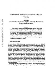
In Fig. 3, we have plotted the solution to this gap equation normalized to the leading-order perturbative result in (4) as a function of αs (2πT ). The shaded band indicates the range resulting from varying the renormalization scale µ by a factor of two around µ = 2πT . From this plot, we see that the gap equation solution matches nicely onto the perturbative result as αs → 0. The solution decreases with αs (2πT ) out to about αs ≈ 0.06 and then begins to increase. It exceeds the perturbative result at around αs ≈ 0.18, and then quickly diverges to +∞. VII. THERMODYNAMIC FUNCTIONS

In this section, we compare the thermodynamic functions calculated at next-to-leading order in HTL perturbation theory (HTLpt) with those calculated using lattice gauge theory.

19

FIG. 3. Solution to the gap equation (63) as a function of αs (2πT ). The shaded band corresponds to variation of the renormalization scale µ by a factor of two around µ = 2πT . A. Pressure

The final results for the LO and NLO HTLpt predictions for the free energy of pureglue QCD are obtained by evaluating the thermodynamic potentials (56) and (62) at the solution to the gap equation (63). Once the free energy F (T ) is given as a function of T , all other thermodynamic functions are determined. In particular, the pressure P and the energy density E are P = −F ,

dF E =F −T . dT

(64) (65)

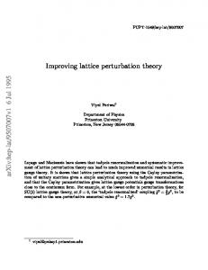
In Figure 4, we have plotted the LO and NLO HTLpt predictions for the pressure of pureglue QCD as a function of T /Tc , where Tc is the deconfinement transition temperature. To translate αs (2πT ) into a value of T /Tc , we use the two-loop running formula for pure-glue QCD with ΛMS = 0.65 Tc . Thus αs (2πT ) = 0.06 and 0.2 translate into T /Tc = 415 and 0.906, respectively. The LO and NLO HTLpt results are shown in Fig. 4 as a light-shaded band outlined by a dashed line and a dark-shaded band outlined by a solid line, respectively. The LO and NLO bands overlap all the way down to T = Tc , and the bands are very narrow compared to the corresponding bands for the weak-coupling predictions in Fig. 1. Thus the convergence of HTLpt seems to be dramatically improved over naive perturbation theory and the final result is extremely insensitive to the scale µ. In Fig. 4, we have also included the 4-dimensional lattice gauge theory results of Boyd et al. [5] and the 3-dimensional lattice gauge theory results of Kajantie et al. [7]. The LO 20

FIG. 4. The LO and NLO results for the pressure in HTLpt compared with 4-d lattice results (diamonds) and 3-d lattice results (dotted lines) for various values of an unknown coefficient in the 3-d effective Lagrangian. The LO HTLpt result is shown as a light-shaded band outlined by a dashed line. The NLO HTLpt result is shown as a dark-shaded band outlined by a solid line. The shaded bands correspond to variations of the renormalization scale µ by a factor of two around µ = 2πT .

and NLO HTLpt predictions differ significantly from the 4-d lattice results of Ref. [5], even at the highest temperatures for which they are available. At T = 5 Tc , the HTLpt prediction for the deviation of the pressure from that of the ideal gas is only 45% of the 4-d lattice result. In the high temperature limit, the HTLpt prediction approaches that of the ideal gas very slowly, in qualitative agreement with the results of the 3-d lattice calculations of Ref. [7]. However the quantitative agreement is not very good. The results of Ref. [7] depend on an unknown coefficient in the effective lagrangian for the dimensionally reduced theory. The 5 dotted lines in Fig. 4 correspond to 5 possible values for that coefficient. We assume that the coefficient is such that the 3-d results match on reasonably well to the 4-d results, such as one of the middle 3 of the 5 dotted lines. In that case, the HTLpt prediction for the deviation from the ideal gas at T = 103 Tc is only about 59% of the 3-d lattice result. We conclude that HTLpt at this order does not describe the pressure for pure-glue QCD. B. Trace Anomaly

The combination E − 3P can be written as d E − 3P = −T dT 5

21



F . T4 

(66)

This combination is proportional to the trace of the energy-momentum tensor. In QCD with massless quarks, it is nonzero only because scale invariance is broken by renormalization effects. We will call it the trace anomaly density. It of course vanishes for an ideal gas of massless particles. However, it also vanishes for a gas of quasiparticles whose masses are linear in T and whose interactions are governed by a dimensionless coupling constant that is independent of T .

FIG. 5. The LO and NLO results for the trace anomaly in HTLpt. The LO HTLpt result is shown as a light-shaded band outlined by a dashed line. The NLO HTLpt result is shown as a dark-shaded band outlined by a solid line. The shaded bands correspond to variations of the renormalization scale µ by a factor of two around µ = 2πT .

In Fig. 5, we have plotted the LO and NLO HTLpt predictions for the trace anomaly density as a function of T /Tc . At large T , the HTLpt prediction is very small and positive. As T decreases, the NLO prediction for E − 3P increases to its maximum value around 10Tc and then begins decreasing and quickly turns negative. The maximum value is less than about 0.2% of the energy density Eideal of the ideal gas. In contrast, the 4-d lattice result increases to a maximum of about 70% of Eideal at a temperature that is very close to Tc and then decreases rapidly to 0 [5]. VIII. CONCLUSIONS

We have calculated the free energy of pure-glue QCD at high temperature to 2-loop order using HTL perturbation theory (HTLpt). The gauge invariance of the 2-loop expression was verified explicitly in generalized covariant gauge and generalized Coulomb gauge. The expression was reduced to a relatively compact form involving only scalar sum-integrals. 22

The numerical evaluation of the scalar sum-integrals would have been extremely difficult. We chose instead to approximate them by expanding in powers of mD /T , keeping all terms through 5th order in g and mD /T . The ultraviolet divergences in the resulting expression for the thermodynamic potential can be removed by renormalization of the vacuum energy density and the HTL mass parameter mD . This provides a nontrivial test of the renormalizability of HTL perturbation theory to this order. The two-loop order of HTLpt is the first order at which mD can be determined by a variational prescription. The condition that mD be a stationary point of the thermodynamic potential provides a “gap equation” for mD . The only ambiguity in the free energy then resides in the scale µ associated with renormalizations of the vacuum energy density and mD . The predictions for the thermodynamic functions are extremely insensitive to the choice of µ. The quantitative predictions for the pressure in 2-loop HTLpt are disappointing. In the range 2Tc < T < 20Tc , the pressure is predicted to be nearly constant with a value of about 95% of that of an ideal gas of gluons. The HTLpt prediction for the deviation from the ideal gas is about 45% of the result from 4-dimensional lattice gauge theory at T = 5Tc , the highest temperature for which the lattice result is available. At very high temperature, the approach to the ideal gas limit is extremely slow, in qualitative agreement with the results of 3-d lattice gauge theory calculations. However, assuming that the 3-d results match on reasonably well to the 4-d results, the HTLpt prediction for the deviation from the ideal gas at T = 103 Tc is only about 59% of the 3-d lattice result. A possible conclusion is that HTLpt at two-loop order is simply not a useful approximation for thermal QCD. Another possibility is that the problem lies not with HTLpt but with our use of the mD /T expansion to approximate the scalar sum-integrals. The sum-integrals that were encountered at 4th and 5th order in mD /T were so difficult to evaluate that it seems hopeless to try to expand to higher order. However it is possible that the scalar sum-integrals could be evaluated numerically. Part of the difficulty is that it is necessary to isolate the infrared divergent and ultraviolet divergent terms analytically before evaluating the remaining terms numerically. Our mD /T expansions of the sum-integrals might be useful for generating the necessary subtractions that would allow the scalar sum-integrals to be evaluated numerically. Our calculations required the development of new methods for evaluating sum-integrals. The most difficult were two-loop sum-integrals that also involved an HTL angular average. These sum-integrals may be useful in other applications, such as solving the 2-loop Φderivable approximation for QCD. IX. ACKNOWLEDGEMENTS

E.B. and E.P. were supported in part by Department of Energy grant DE-FG02-91ER4069. J.O.A. was supported by the Stichting voor Fundamenteel Onderzoek der Materie (FOM), which is supported by the Nederlandse Organisatie voor Wetenschapplijk Onderzoek (NWO). M.S. was supported by US DOE Grants DE-FG02-96ER40945 and DE-FG0397ER41014.

23

APPENDIX A: HTL FEYNMAN RULES

In this appendix, we present Feynman rules for HTL perturbation theory in pure-glue QCD. We give explicit expressions for the propagators and for the 3-particle and 4-particle vertices. The Feynman rules are given in Minkowski space to facilitate applications to realtime processes. A Minkowski momentum is denoted p = (p0 , p), and the inner product is p · q = p0 q0 − p · q. The vector that specifies the thermal rest frame is n = (1, 0). 1. Gluon Self-energy

The HTL gluon self-energy tensor for a gluon of momentum p is Πµν (p) = m2D [T µν (p, −p) − nµ nν ] .

(A.1)

The tensor T µν (p, q), which is defined only for momenta that satisfy p + q = 0, is T

µν

*

µ ν p·n

(p, −p) = y y

p·y

+

.

(A.2)

y ˆ

The angular brackets indicate averaging over the spatial directions of the light-like vector ˆ ). The tensor T µν is symmetric in µ and ν and satisfies the “Ward identity” y = (1, y pµ T µν (p, −p) = p·n nν .

(A.3)

The self-energy tensor Πµν is therefore also symmetric in µ and ν and satisfies pµ Πµν (p) = 0 , gµν Πµν (p) = −m2D .

(A.4) (A.5)

The gluon self-energy tensor can be expressed in terms of two scalar functions, the transverse and longitudinal self-energies ΠT and ΠL , defined by  1  ij δ − pˆi pˆj Πij (p) , d−1 ΠL (p) = −Π00 (p) ,

ΠT (p) =

(A.6) (A.7)

where p ˆ is the unit vector in the direction of p. In terms of these functions, the self-energy tensor is Πµν (p) = −ΠT (p)Tpµν −

1 ΠL (p)Lµν p , n2p

(A.8)

where the tensors Tp and Lp are Tpµν = g µν − Lµν p =

nµp nνp pµ pν , − p2 n2p

nµp nνp . n2p

(A.9) (A.10)

24

The four-vector nµp is nµp = nµ −

n·p µ p p2

(A.11)

and satisfies p·np = 0 and n2p = 1 − (n·p)2 /p2 . The equation (A.5) reduces to the identity (d − 1)ΠT (p) +

1 ΠL (p) = m2D . n2p

(A.12)

We can express both self-energy functions in terms of the function T 00 defined by (A.2): ΠT (p) =

h i m2D 00 2 T (p, −p) − 1 + n p , (d − 1)n2p h

i

ΠL (p) = m2D 1 − T 00 (p, −p) ,

(A.13) (A.14)

In the tensor T µν (p, −p) defined in (A.2), the angular brackets indicate the angular ˆ . In almost all previous work, the angular average in (A.2) average over the unit vector y has been taken in d = 3 dimensions. For consistency of higher order radiative corrections, it is essential to take the angular average in d = 3 − 2ǫ dimensions and analytically continue to d = 3 only after all poles in ǫ have been cancelled. Expressing the angular average as an integral over the cosine of an angle, the expression for the 00 component of the tensor is T

00

w(ǫ) (p, −p) = 2

Z

1 −1

dc (1 − c2 )−ǫ

p0 , p0 − |p|c

(A.15)

where the weight function w(ǫ) is Γ( 23 − ǫ) Γ(2 − 2ǫ) 2ǫ . 2 = 3 w(ǫ) = 2 Γ (1 − ǫ) Γ( 2 )Γ(1 − ǫ)

(A.16)

The integral in (A.15) must be defined so that it is analytic at p0 = ∞. It then has a branch cut running from p0 = −|p| to p0 = +|p|. If we take the limit ǫ → 0, it reduces to T 00 (p, −p) =

p0 p0 + |p| log , 2|p| p0 − |p|

(A.17)

which is the expression that appears in the usual HTL self-energy functions. 2. Gluon Propagator

The Feynman rule for the gluon propagator is iδ ab ∆µν (p) ,

(A.18)

where the gluon propagator tensor ∆µν depends on the choice of gauge fixing. We consider two possibilities that introduce an arbitrary gauge parameter ξ: general covariant gauge and 25

general Coulomb gauge. In both cases, the inverse propagator reduces in the limit ξ → ∞ to µν ∆−1 = −p2 g µν + pµ pν − Πµν (p) . ∞ (p)

(A.19)

This can also be written µν ∆−1 =− ∞ (p)

1 1 Tpµν + 2 Lµν , ∆T (p) np ∆L (p) p

(A.20)

where ∆T and ∆L are the transverse and longitudinal propagators: 1 ∆T (p) = 2 , p − ΠT (p) 1 . ∆L (p) = −n2p p2 + ΠL (p) The inverse propagator for general ξ is 1 µν ∆−1 (p)µν = ∆−1 − pµ pν ∞ (p) ξ 1 µν = ∆−1 − (pµ − p·n nµ ) (pν − p·n nν ) ∞ (p) ξ

(A.21) (A.22)

covariant ,

(A.23)

Coulomb .

(A.24)

The propagators obtained by inverting the tensors in (A.24) and (A.23) are ∆µν (p) = −∆T (p)Tpµν + ∆L (p)nµp nνp − ξ

pµ pν (p2 )2 pµ pν

= −∆T (p)Tpµν + ∆L (p)nµ nν − ξ 

n2p p2

2

covariant ,

(A.25)

Coulomb .

(A.26)

It is convenient to define the following combination of propagators: 1 ∆X (p) = ∆L (p) + 2 ∆T (p) . np

(A.27)

Using (A.12), (A.21), and (A.22), it can be expressed in the alternative form h

i

∆X (p) = m2D − d ΠT (p) ∆L (p)∆T (p) ,

(A.28)

which shows that it vanishes in the limit mD → 0. In the covariant gauge, the propagator tensor can be written n·p ∆µν (p) = [−∆T (p)g µν + ∆X (p)nµ nν ] − 2 ∆X (p) (pµ nν + nµ pν ) p " # 2 (n·p) ξ pµ pν + ∆T (p) + ∆X (p) − 2 . (A.29) p2 p p2 This decomposition of the propagator into three terms has proved to be particularly convenient for explicit calculations. For example, the first term satisfies the identity νλ [−∆T (p)gµν + ∆X (p)nµ nν ] ∆−1 = gµ λ − ∞ (p)

26

pµ pλ n·p ∆X (p) + pµ nλp . 2 2 2 p np p ∆L (p)

(A.30)

3. Three-gluon Vertex

The three-gluon vertex for gluons with outgoing momenta p, q, and r, Lorentz indices µ, ν, and λ, and color indices a, b, and c is µνλ iΓµνλ (p, q, r) , abc (p, q, r) = −gfabc Γ

(A.31)

where the three-gluon vertex tensor is Γµνλ (p, q, r) = g µν (p − q)λ + g νλ (q − r)µ + g λµ (r − p)ν − m2D T µνλ (p, q, r) .

(A.32)

The tensor T µνλ in the HTL correction term is defined only for p + q + r = 0: *

T µνλ (p, q, r) = − y µ y ν y λ

p·n r·n − p·y q·y r ·y q·y

!+

.

(A.33)

This tensor is totally symmetric in its three indices and traceless in any pair of indices: gµν T µνλ = 0. It is odd (even) under odd (even) permutations of the momenta p, q, and r. It satisfies the “Ward identity” qµ T µνλ (p, q, r) = T νλ (p + q, r) − T νλ (p, r + q) .

(A.34)

The three-gluon vertex tensor therefore satisfies the Ward identity νλ νλ pµ Γµνλ (p, q, r) = ∆−1 − ∆−1 . ∞ (q) ∞ (r)

(A.35)

4. Four-gluon Vertex

The four-gluon vertex for gluons with outgoing momenta p, q, r, and s, Lorentz indices µ, ν, λ, and σ, and color indices a, b, c, and d is iΓµνλσ abcd (p, q, r, s)

(



= −ig 2 fabx fxcd g µλ g νσ − g µσ g νλ +2m2D tr

h

T

a



b

c

d

d

 c

T T T +T T T

+ 2 cyclic permutations ,

b

i

T

µνλσ

(p, q, r, s)

)

(A.36)

where the cyclic permutations are of (q, ν, b), (r, λ, c), and (s, σ, d). The matrices T a are the fundamental representation of the SU(3) algebra with the standard normalization tr(T a T b ) = 21 δ ab . The tensor T µνλσ in the HTL correction term is defined only for p + q + r + s = 0: T

µνλσ

*

p·n p·y q·y (q + r)·y !+ (p + q)·n (p + q + r)·n + . + q·y r·y (r + s)·y r·y s·y (s + p)·y

(p, q, r, s) = y µ y ν y λ y σ

27

(A.37)

This tensor is totally symmetric in its four indices and traceless in any pair of indices: gµν T µνλσ = 0. It is even under cyclic or anti-cyclic permutations of the momenta p, q, r, and s. It satisfies the “Ward identity” qµ T µνλσ (p, q, r, s) = T νλσ (p + q, r, s) − T νλσ (p, r + q, s)

(A.38)

and the “Bianchi identity” T µνλσ (p, q, r, s) + T µνλσ (p, r, s, q) + T µνλσ (p, s, q, r) = 0 .

(A.39)

When its color indices are traced in pairs, the four-gluon vertex becomes particularly simple: 2 2 µν,λσ δ ab δ cd iΓµνλσ (p, q, r, s) , abcd (p, q, r, s) = −ig Nc (Nc − 1)Γ

(A.40)

where the color-traced four-gluon vertex tensor is Γµν,λσ (p, q, r, s) = 2g µν g λσ − g µλ g νσ − g µσ g νλ − m2D T µνλσ (p, s, q, r) .

(A.41)

Note the ordering of the momenta in the arguments of the tensor T µνλσ , which comes from the use of the Bianchi identity (A.39). The tensor (A.41) is symmetric under the interchange of µ and ν, under the interchange of λ and σ, and under the interchange of (µ, ν) and (λ, σ). It is also symmetric under the interchange of p and q, under the interchange of r and s, and under the interchange of (p, q) and (r, s). It satisfies the Ward identity pµ Γµν,λσ (p, q, r, s) = Γνλσ (q, r + p, s) − Γνλσ (q, r, s + p) .

(A.42)

5. Ghost propagator and vertex

The ghost propagator and the ghost-gluon vertex depend on the gauge. The Feynman rule for the ghost propagator is i ab δ p2 i ab δ 2 np p2

covariant ,

(A.43)

Coulomb .

(A.44)

The Feynman rule for the vertex in which a gluon with indices µ and a interacts with an outgoing ghost with outgoing momentum r and color index c is −gf abc r µ −gf abc (r µ − r·n nµ )

covariant , Coulomb .

Every closed ghost loop requires a multiplicative factor of −1. 28

(A.45) (A.46)

6. HTL Counterterm

The Feynman rule for the insertion of an HTL counterterm into a gluon propagator is − iδ ab Πµν (p) ,

(A.47)

where Πµν (p) is the HTL gluon self-energy tensor given in (A.8). 7. Imaginary-time formalism

In the imaginary-time formalism, Minkoswski energies have discrete imaginary values p0 = i(2πnT ) and integrals over Minkowski space are replaced by sum-integrals over Euclidean vectors (2πnT, p). We will use the notation P = (P0 , p) for Euclidean momenta. The magnitude of the spatial momentum will be denoted p = |p|, and should not be confused with a Minkowski vector. The inner product of two Euclidean vectors is P · Q = P0 Q0 + p· q. The vector that specifies the thermal rest frame remains n = (1, 0). The Feynman rules for Minkowski space given above can be easily adapted to Euclidean space. The Euclidean tensor in a given Feynman rule is obtained from the corresponding Minkowski tensor with raised indices by replacing each Minkowski energy p0 by iP0 , where P0 is the corresponding Euclidean energy, and multipying by −i for every 0 index. This prescription transforms p = (p0 , p) into P = (P0 , p), g µν into −δ µν , and p·q into −P ·Q. The effect on the HTL tensors defined in (A.2), (A.33), and (A.37) is equivalent to substituting p · n → −P · N where N = (−i, 0), p · y → −P · Y where Y = (−i, y ˆ), and y µ → Y µ . For example, the Euclidean tensor corresponding to (A.2) is 

T µν (P, −P ) = Y µ Y ν

P ·N P ·Y



.

(A.48)

The average is taken over the directions of the unit vector y ˆ. Alternatively, one can calculate a diagram by using the Feynman rules for Minkowski momenta, reducing the expressions for diagrams to scalars, and then make the appropriate substitutions, such as p2 → −P 2 , p · q → −P · Q, and n · p → in · P . For example, the propagator functions (A.21) and (A.22) become −1 , + ΠT (P ) 1 ∆L (P ) = 2 . p + ΠL (P )

∆T (P ) =

P2

(A.49) (A.50)

The expressions for the HTL self-energy functions ΠT (P ) and ΠL (P ) are given by (A.13) and (A.14) with n2p replaced by n2P = p2 /P 2 and T 00 (p, −p) replaced by w(ǫ) TP = 2

Z

1

−1

dc (1 − c2 )−ǫ

iP0 . iP0 − pc

(A.51)

Note that this function differs by a sign from the 00 component T 00 (P, −P ) of the Euclidean tensor corresponding to (A.2): 29



T 00 (P, −P ) = −T 00 (p, −p)

p0 →iP0

= −TP .

(A.52)

A more convenient form for calculating sum-integrals that involve the function TP is TP =

*

P02 P02 + p2 c2

+

,

(A.53)

c

where the angular brackets represent an average over c defined by hf (c)ic ≡ w(ǫ)

Z

0

1

dc (1 − c2 )−ǫ f (c)

(A.54)

and w(ǫ) is given in (A.16). APPENDIX B: SUM-INTEGRALS

In the imaginary-time formalism for thermal field theory, a boson has Euclidean 4momentum P = (P0 , p), with P 2 = P02 + p2 . The Euclidean energy P0 has discrete values: P0 = 2πnT , where n is an integer. Loop diagrams involve sums over P0 and integrals over p. With dimensional regularization, the integral is generalized to d = 3 − 2ǫ spatial dimensions. We define the dimensionally regularized sum-integral by Z P

P

≡

eγ µ2 4π

!ǫ

T

X Z P0

d3−2ǫ p , (2π)3−2ǫ

(B.1)

where d = 3−2ǫ is the dimension of space and µ is an arbitrary momentum scale. The factor (eγ /4π)ǫ is introduced so that, after minimal subtraction of the poles in ǫ due to ultraviolet divergences, µ coincides with the renormalization scale of the MS renormalization scheme. 1. Simple one-loop sum-integrals

The simple one-loop sum-integrals required in our calculations are π2 4 T , 45 P " ! #   Z ζ ′(−1) µ 2ǫ 1 P 1 2 1+ 2+2 ǫ , =T 4πT 12 ζ(−1) P P2 Z 1 2 P p2 = T , 8 P (P 2 )2 ! # "   Z 1 1 π2 µ 2ǫ 1 P = + 2γ + 2 + 4 + 4γ + − 4γ1 ǫ , 2 (4π)2 4πT ǫ 4 P p2 P 2 ! #  "  Z 1 µ 2ǫ 1 π2 1 P = + 2γ + − 4γ1 ǫ , (4π)2 4πT ǫ 4 P (P 2 )2

Z P

log P 2 = −

30

(B.2) (B.3) (B.4) (B.5) (B.6)

Z P

P

Z P

P

Z P

P

1 p2 µ 2ǫ = (P 2 )3 (4π)2 4πT   1 µ 2ǫ p4 = (P 2 )4 (4π)2 4πT 1 2ζ(3) 1 = . 2 3 (P ) (4π)4 T 2 



3 1 + 2γ − 4 ǫ  5 1 + 2γ − 8 ǫ 

2 , 3  16 , 15 

(B.7) (B.8) (B.9)

The calculation of these sum-integrals is standard. The errors are all one order higher in ǫ than the smallest term shown. The number γ1 is the first Stieltjes gamma constant defined by the equation ζ(1 + z) =

1 + γ − γ1 z + O(z 2 ) . z

(B.10)

2. One-loop HTL sum-integrals

The one-loop sum-integrals involving the HTL function TP defined in (A.51) are 1 TP P P2 Z P 1 TP P p4 Z 1 P TP 2 P p P2 Z 1 P TP P (P 2 )2 Z P 1 (TP )2 P p4 Z P

=T

2



1 (4π)2 1 = (4π)2 1 = (4π)2 1 = (4π)2 =

"

#

1 ζ ′(−1) , +2 ǫ ζ(−1)     µ 2ǫ 1 + 2γ + 2 log 2 , (−1) 4πT ǫ # 2ǫ "    1 π2 µ 2 2 log 2 , + 2γ + 2 log 2 + 4πT ǫ 3     µ 2ǫ 1 1 + 2γ + 1 , 4πT 2 ǫ       2 1 µ 2ǫ − (1 + 2 log 2) + 2γ 4πT 3 ǫ  4 22 2 log 2 + 2 log 2 . − + 3 3

µ 4πT

2ǫ 

1 − 24

(B.11) (B.12) (B.13) (B.14)

(B.15)

The errors are all of order ǫ. It is straightforward to calculate the sum-integrals (B.11)–(B.15) using the representation (A.53) of the function TP . For example, the sum-integral (B.11) can be written Z P

P

1 1 P TP = 2 2 P P P 0 + p2 Z

*

P02 P02 + p2 c2

+

,

(B.16)

c

where the angular brackets denote an average over c as defined in (A.54). Using the factor of P02 in the numerator to cancel denominators, this becomes Z P

P

1 TP = P2

*

1 P 1 − c2 P Z

1 c2 − P 2 P02 + p2 c2 31

!+

c

.

(B.17)

After rescaling the momentum by p → p/c, the second sum-integral on the right side becomes the same as the first sum-integral, and the expression reduces to 1 TP = P2

Z P

P

*

1 − c−1+2ǫ 1 − c2

+Z P c

P

1 . P2

(B.18)

Evaluating the average over c, using the expression (B.3) for the sum-integral, and expanding in powers of ǫ, we obtain the result (B.11). Following the same strategy, all the sum-integrals (B.11)–(B.15) can be reduced to linear combinations of the simple sum-integrals (B.3) and (B.5) with coefficients that are averages over c. The only difficult integral is the double average over c that arises from (B.15): *

c3+2ǫ − c3+2ǫ 1 2 2 2 c1 − c2

+

c1 ,c2

10 10 2 1 + 2 log 2 + − + log 2 + log2 2 ǫ . = 3 9 9 3 



(B.19)

3. Simple two-loop sum-integrals

The simple two-loop sum-integrals that are needed are 1 P Q P 2 Q2 R2 Z 1 P 2 P Q P Q2 r 2 Z q2 P P Q P 2 Q2 r 4 Z q2 P P Q P 2 Q2 r 2 R2 Z P ·Q P P Q P 2 Q2 r 4 Z P

= 0, = = = =

(B.20)

T2 ζ ′ (−1) µ 4ǫ 1 1 , + 10 − 12 log 2 + 4 (4π)2 4πT 12 ǫ ζ(−1) " #   T2 ζ ′ (−1) µ 4ǫ 1 1 8 , + + 2γ + 2 (4π)2 4πT 6 ǫ 3 ζ(−1)     T2 µ 4ǫ 1 1 + 7.521 , (4π)2 4πT 9 ǫ #   "  1 1 2 T2 8 4 ζ ′(−1) µ 4ǫ − , + + 4 log 2 + γ + (4π)2 4πT 8 ǫ 9 3 3 ζ(−1) "





#

(B.21) (B.22) (B.23) (B.24)

where R = −(P + Q) and r = |p + q|. The errors are all of order ǫ. To motivate the integration formula we will use to evaluate the two-loop sum-integrals, we first present the analogous integration formula for one-loop sum-integrals. In a one-loop sum-integral, the sum over P0 can be replaced by a contour integral in p0 = −iP0 : Z P

P

F (P ) = lim+ η→0

Z

dp0 2πi

Z

p

[F (−ip0 , p) − F (0, p)] eηp0 n(p0 ) ,

(B.25)

where n(p0 ) = 1/(eβp0 − 1) is the Bose-Einstein thermal distribution and the contour runs from −∞ to +∞ above the real axis and from +∞ to −∞ below the real axis. This formula can be expressed in a more convenient form by collapsing the contour onto the real axis and separating out those terms with the exponential convergence factor n(|p0 |). The remaining terms run along contours from −∞ ± iε to 0 and have the convergence factor eηp0 . This allows the contours to be deformed so that they run from 0 to ±i∞ along the imaginary 32

p0 axis, which corresponds to real values of P0 = −ip0 . Assuming that F (−ip0 , p) is a real function of p0 , i.e. that it satisfies F (−ip∗0 , p) = F (−ip0 , p)∗ , the resulting formula for the sum-integral is Z P

P

Z

F (P ) =

P

F (P ) +

Z

p

ǫ(p0 )n(|p0 |) 2ImF (−ip0 + ε, p) ,

(B.26)

where ǫ(p0 ) is the sign of p0 . The first integral on the right side is over the (d+1)-dimensional Euclidean vector P = (P0 , p) and the second is over the (d + 1)-dimensional Minkowskian vector p = (p0 , p). The two-loop sum-integrals can be evaluated by using a generalization of the one-loop formula (B.26): 1 F (P )G(Q)H(R) = 3 PQ

Z P

+ +

Z

p

Z

p

Z

PQ

F (P )G(Q)H(R)

ǫ(p0 )n(|p0 |) 2ImF (−ip0 + ε, p) Re ǫ(p0 )n(|p0 |) 2ImF (−ip0 + ε, p) ×ReH(R)

Z

G(Q)H(R)

Z

Q

P0 =−ip0 +ε

ǫ(q0 )n(|q0 |) 2ImG(−iq0 + ε, q)

q

+ (cyclic permutations of F, G, H) .

(B.27)

R0 =i(p0 +q0 )+ε

The sum over cyclic permutations multiplies the first term on the right side by 3, so there are a total of 7 terms. This formula can be derived in 3 steps. First, express the sum over P0 as the sum of two contour integrals over p0 , one that encloses the real axis Im p0 = 0 and another that encloses the line Im p0 = −Im q0 . Second, express the sum over q0 as a contour integral that encloses the real-q0 axis. Third, symmetrize the resulting expression under the 6 permutations of F , G, and H. The resulting terms can be combined into the expression (B.27). The integrals of the imaginary parts that enter into our calculation can be reduced to 1 f (−ip0 + ε, p) = ǫ(p0 )n(|p0 |) 2Im 2 P P0 =−ip0 +ε p

Z



Z

ǫ(p0 )n(|p0 |) 2ImTP

p

P0 =−ip0 +ε

Z

p

n(p) 1 X f (±ip + ε, p) , p 2 ±

(B.28)

f (−ip0 + ε, p) =−

Z

p n(p)

p

E 1 X D −3+2ǫ c f (±ip + ε, p/c) . c 2 ±

(B.29)

The latter equation is obtained by inserting the expression (A.53) for TP , using (B.28), and then making the change of variable p → p/c to put the thermal integral into a standard form. As a simple illustration, we apply the formula (B.27) to the sum-integral (B.21). The nonvanishing terms are Z P

PQ

1 =2 2 P Q2 r 2

Z

+

p

n(|p0 |) 2πδ(p20 − p2 ) Z

p

n(|p0 |) 2πδ(p20

Q Q2 r 2

2

−p ) 33

1

Z

Z

q

n(|q0 |) 2πδ(q02 − q 2 )

1 . r2

(B.30)

The delta functions can be used to evaluate the integrals over p0 and q0 . The integral over Q is given in (C.98) up to corrections of order ǫ. This reduces the sum-integral to Z P

PQ

1 4 1 = + 4 − 2 log 2 µ2ǫ 2 2 2 2 P Qr (4π) ǫ 



Z

p

n(p) −2ǫ p + p

Z

pq

n(p)n(q) 1 . pq r2

(B.31)

The momentum integrals are evaluated in (C.5) and (C.6). Keeping all terms that contribute through order ǫ0 , we get the result (B.21). The sum-integral (B.22) can be evaluated in the same way: Z P

PQ

2 1 q2 = − 2 log 2 µ2ǫ 2 2 4 2 P Qr (4π) ǫ 



Z

p

n(p) −2ǫ p + p

Z

pq

n(p)n(q) q 2 . pq r4

(B.32)

The sum-integral (B.24) can be reduced to a linear combination of (B.21) and (B.22) by expressing the numerator in the form P ·Q = P0 Q0 + (r 2 − p2 − q 2 )/2 and noting that the P0 Q0 term vanishes upon summing over P0 or Q0 . The sum-integral (B.23) is a little more difficult. After applying the formula (B.27) and using the delta functions to integrate over p0 , q0 , and r0 , it can be reduced to Z P

PQ

q2 = P 2 Q2 r 2 R2

n(p) p

Z

p

+

Z

pq

1 p2 q 2 q 2 + + r 2 r 2 p2 P0 =−ip Q Q2 R2 ! n(p)n(q) p2 p2 r 2 r 2 − p2 − q 2 + + , pq r2 q2 q2 ∆(p, q, r) !

Z

(B.33)

where ∆(p, q, r) is the triangle function that is negative when p, q, and r are the lengths of 3 sides of a triangle: ∆(p, q, r) = p4 + q 4 + r 4 − 2(p2 q 2 + q 2 r 2 + r 2 p2 ) .

(B.34)

After using (C.104)–(C.106) to integrate over Q, the first term on the right side of (B.33) is evaluated using (C.5). The 2-loop thermal integrals on the right side of (B.33) are given in (C.8)–(C.11). Adding together all the terms, we get the final result (B.23). 4. Two-loop HTL sum-integrals

The two-loop sum-integrals involving the HTL function TP defined in (A.51) are Z P

PQ

Z P

PQ

1 T2 T = R P 2 Q2 r 2 (4π)2

4ǫ 

1 48

1 ǫ2 ! # ζ ′(−1) 1 − 19.83 , + 2 − 12 log 2 + 4 ζ(−1) ǫ     q2 1 1 T2 µ 4ǫ − TR = 2 2 4 2 P Qr (4π) 4πT 576 ǫ2 ! # ζ ′(−1) 1 26 24 + − 2 − 92 log 2 + 4 − 477.7 , 3 π ζ(−1) ǫ 

µ 4πT

−



34

(B.35)

(B.36)

Z P

PQ

T2 P ·Q T = R P 2 Q2 r 4 (4π)2

1 1 µ 4ǫ − 4πT 96 ǫ2 ! # 8 ζ ′(−1) 1 + + 4 log 2 + 4 + 59.66 . π2 ζ(−1) ǫ 







(B.37)

To calculate the sum-integral (B.35), we begin by using the representation (A.53) of the function TR : Z P

PQ

1 1 1 P P T = − R P 2 Q2 r 2 P Q P 2 Q2 r 2 P Q P 2 Q2 Z

Z

*

c2 R02 + r 2 c2

+

.

(B.38)

c

The first sum-integral on the right side is given by (B.21). To evaluate the second sumintegral, we apply the sum-integral formula (B.27): 1

Z P

2 P Q P 2 Q2 (R0

+ r 2 c2 ) ! Z Z Z n(p) 1 1 −3+2ǫ = +c 2Re 2 p p Q Q2 R2 P →(−ip,p/c) Q Q2 (R0 + r 2 c2 ) P0 =−ip+ε ! Z n(p)n(q) r 2 c2 − p 2 − q 2 rc2 − p2 − q 2 −3+2ǫ + Re , + 2c Re pq ∆(p + iε, q, rc) ∆(p + iε, q, rc ) pq

(B.39)

where rc = |p + q/c|. In the terms on the right side with a single thermal integral, the appropriate averages over c of the integrals over Q are given in (C.109) and (C.102). *

c

2

2Re

Z

Q

Z 1 1 −3+2ǫ + c Q2 (R02 + r 2 c2 ) P0 =−ip+ε Q Q2 R2 P →(−ip,p/c)



!+

c

1 1 7 13π 2 17 1 2ǫ −2ǫ = µ p + 4 − log 2 + 16 − − 8 log 2 + log2 2 . 2 2 (4π) 4ǫ 2 ǫ 16 2 "



#



(B.40)

The subsequent integral over p is a special case of (C.5): Z

n(p) p

−1−2ǫ

p

2 (1)−4ǫ ( 12 )2ǫ ζ(−1 + 4ǫ) γ 2 ǫ −4ǫ T (e µ ) (4πT ) , =2 (1)−2ǫ ( 32 )−ǫ ζ(−1) 12 8ǫ

(B.41)

where (a)b = Γ(a+b)/Γ(a) is Pochhammer’s symbol. Combining this with (B.40), we obtain Z

n(p) 2 Re p p 2

=

T (4π)2



Z

Q

µ 4πT

1 Q2

4ǫ

*

c2 R02 + r 2 c2 "

+

*

+ c

c P0 =−ip+ε

−1+2ǫ

′

1 1 ζ (−1) + 18 − 12 log 2 + 4 2 48 ǫ ζ(−1)

Z

Q

!

1 2 Q R2 P →(−ip,p/c)

+! c

#

1 + 173.30233 . ǫ

(B.42)

For the two terms in (B.39) with a double thermal integral, the averages weighted by c2 are given in (C.12) and (C.15). Adding them to (B.42), the final result is 1 2 P Q P Q2

Z P

*

c2 R02 + r 2 c2

+

c

T2 = (4π)2



µ 4πT

4ǫ

1 1 48 ǫ2

+

ζ ′(−1) 6 − 12 log 2 + 4 ζ(−1)



35

!

#

1 + 18.66 . ǫ

(B.43)

Inserting this into (B.38), we obtain the final result (B.35). The sum-integral (B.36) is evaluated in a similar way to (B.35). Using the representation (A.53) for TR , we get Z Z q2 q2 q2 P P T = − R P 2 Q2 r 4 P Q P 2 Q2 r 4 P Q P 2 Q2 r 2

Z P

PQ

*

c2 R02 + r 2 c2

+

.

(B.44)

c

The first sum-integral on the right hand side is given by (B.22). To evaluate the second sum-integral, we apply the sum-integral formula (B.27): q2 2 P Q P 2 Q2 r 2 (R0 + r 2 c2 ) ! Z Z Z 1 −1+2ǫ q 2 p2 + q 2 n(p) + 2c Re = 2 p Q Q2 R2 P →(−ip,p/c) Q Q2 r 2 (R0 + r 2 c2 ) P0 =−ip+ε p p ! Z 2 2 n(p)n(q) q 2 r 2 c2 − p 2 − q 2 rc2 − p2 − q 2 −1+2ǫ p + rc + . (B.45) Re +c Re pq r2 ∆(p + iε, q, rc) q2 ∆(p + iε, q, rc ) pq

Z P

In the terms on the right side with a single thermal integral, the weighted averages over c of the integrals over Q are given in (C.112), (C.113), and (C.108): *

c

2

Re

Z

Q

1 p2 + q 2 + 2 c−1+2ǫ 2 2 2 2 2 Q r (R0 + r c ) P0 =−ip+ε p

"

Z

Q

q 2 Q2 R2 P →(−ip,p/c)

!+

c

2

#

1 1 17 65 35 31 1 313 247π = µ2ǫ p−2ǫ + − log 2 + − − log 2 + log2 2 , (B.46) 2 2 (4π) 48ǫ 36 24 ǫ 108 576 18 24 



After using (B.41) to evaluate the thermal integral, we obtain Z

p

n(p) Re p 2

T = (4π)2



Z

Q

µ 4πT

p2 + q 2 Q2 r 2

*

4ǫ

"

c2 R02 + r 2 c2

+ c

*

1 + 2 c1+2ǫ p P0 =−ip+ε ′

ζ (−1) 1 1 146 + − 60 log 2 + 4 2 576 ǫ 3 ζ(−1)

!

Z

Q

q 2 Q2 R2 P →(−ip,p/c)

#

1 + 84.72308 , ǫ

+! c

(B.47)

For the two terms in (B.45) with a double thermal integral, the averages weighted by c2 are given in (C.14), (C.17), and (C.18). Adding them to (B.47), the final result is Z P

PQ

q2 P 2 Q2 r 2

*

c2 R02 + r 2 c2

+

c

=

T2 (4π)2 +



µ 4πT

4ǫ

1 1 576 ǫ2 

314 24 ζ ′(−1) − 2 − 92 log 2 + 4 3 π ζ(−1)

!

#

1 + 270.2 . ǫ

(B.48)

Inserting this into (B.44), we obtain the final result (B.36). To evaluate (B.37), we use the expression (A.53) for TR and the identity P ·Q = (R2 − 2 P − Q2 )/2 to write it in the form Z P

PQ

P ·Q P ·Q P P 1 P 1 TR = − TR 2 2 4 2 2 4 P Qr PQ P Q r P P 2 R r4 * + Z Z 1 2 P 1P c2 (1 − c2 ) 1 1 − hc ic . − 2 2 P Q P 2 Q2 R02 + r 2 c2 c P Q P 2 Q2 r 2 Z

Z

Z

36

(B.49)

The sum-integrals in the first 3 terms on the right side of (B.49) are given in (B.3), (B.12), (B.21), and (B.24). The last sum-integral before the average weighted by c is given in (B.38). The average weighted by c2 is given in (B.43). The average weighted by c4 can be computed in the same way. In the integrand of the single thermal integral, the weighted averages over c of the integrals over Q are given in (C.111) and (C.103): *

!+

1 1 c 2Re + c−3+2ǫ 2 2 2 2 2 Q Q (R0 + r c ) P0 =−ip+ε Q Q R2 P →(−ip,p/c) c    104 23 1 1 µ2ǫ p−2ǫ − 4 log 2 + − π 2 − 3 log 2 + 8 log2 2 , = (4π)2 6 ǫ 9

Z

4



Z

(B.50)

After using (B.41) to evaluate the thermal integral, we obtain n(p) c4 1 + c1+2ǫ 2Re 2 2 2 2 R0 + r c c P0 =−ip+ε p p Q Q 4ǫ    2  23 1 µ 1 T − log 2 + 1.28872 , = (4π)2 4πT 72 3 ǫ

Z

*

Z

*

+

Z

Q

1 Q2 R2 P →(−ip,p/c)

+! c

(B.51)

For the two terms with a double thermal integral, the averages weighted by c4 are given in (C.13) and (C.16). Adding them to (B.51), we obtain Z P

PQ

1 2 P Q2

*

c4 R02 + r 2 c2

+

c

T2 = (4π)2



µ 4πT

4ǫ 

1 1 17 1 − 2 − log 2 − 0.1917 . 72 6π 3 ǫ 



(B.52)

Inserting this into (B.49) along with (B.43), we get the final result (B.37). APPENDIX C: INTEGRALS

Dimensional regularization can be used to regularize both the ultraviolet divergences and infrared divergences in 3-dimensional integrals over momenta. The spatial dimension is generalized to d = 3 − 2ǫ dimensions. Integrals are evaluated at a value of d for which they converge and then analytically continued to d = 3. We use the integration measure Z

p

eγ µ2 4π

≡

!ǫ Z

d3−2ǫ p . (2π)3−2ǫ

(C.1)

1. 3-dimensional integrals

We require several integrals that do not involve the Bose-Einstein distribution function. The momentum scale in these integrals is set by the mass parameter mD . The one-loop integrals are 8 m3 µ 2ǫ 1+ ǫ , log(p + m ) = − 6π 2m 3 p  2ǫ Z 1 m µ =− [1 + 2ǫ] . 2 2 4π 2m p p +m

Z

2

2



37







(C.2) (C.3)

We also require a two-loop integral: Z

pq

1 1 = 2 2 2 2 2 p (q + m )(r + m ) (4π)2



µ 2m

4ǫ

1 1 +2 . 4 ǫ 



(C.4)

The errors in (C.2)–(C.4) are all one order higher in ǫ than the smallest term shown. 2. Thermal integrals

The thermal integrals involve the Bose-Einstein distribution n(p) = 1/(eβp − 1). The one-loop integrals can all be obtained from the general formula Z

p

n(p) 2α ζ(2 + 2α − 2ǫ) Γ(2 + 2α − 2ǫ)Γ( 21 )  γ 2 ǫ 2+2α−2ǫ e µ T . p = p 4π 2 Γ( 23 − ǫ)

(C.5)

The simple two-loop thermal integrals that we need are n(p)n(q) pq pq Z n(p)n(q) pq pq Z

1 1 14 T2 ζ ′ (−1) µ 4ǫ 1 − , = + + 4 log 2 + 4 r2 (4π)2 4πT 4 ǫ 3 ζ(−1) #  "  T2 1 ζ ′(−1) p2 µ 4ǫ 1 1 = + γ− − 4.855 ǫ , r4 (4π)2 4πT 9 3 3 ζ(−1) 





"

#

(C.6) (C.7)

We also need some more complicated 2-loop thermal integrals that involve the triangle function defined in (B.34): T2 r4 n(p)n(q) = pq q 2 ∆(p, q, r) (4π)2

"

!

ζ ′(−1) ζ(3) 7 1 22 + + 2γ + 2 − 48 ǫ2 7 ζ(−1) 35 pq + 40.3896] , " ! 4ǫ Z 2  2 1 1 T ζ ′ (−1) 1 µ n(p)n(q) r = +2 1+γ+ pq ∆(p, q, r) (4π)2 4πT 24 ǫ2 ζ(−1) ǫ pq # π2 ζ ′ (−1) ζ ′′(−1) +4 + 4γ + , − 4γ1 + 4(1 + γ) +2 2 ζ(−1) ζ(−1) !" #   Z ζ(3) T2 1 ζ ′ (−3) ζ ′(3) p4 µ 4ǫ n(p)n(q) − , = +2+2 +2 pq q 2 ∆(p, q, r) (4π)2 4πT 240 ǫ ζ(−3) ζ(3) pq " !   Z n(p)n(q) p2 p2 + q 2 T2 ζ ′(−1) 1 µ 4ǫ 1 1 14 = + + 10γ − 6 pq r 2 ∆(p, q, r) (4π)2 4πT 48 ǫ2 3 ζ(−1) ǫ pq − 86.46] . Z



µ 4πT

4ǫ

1 ǫ (C.8)

(C.9) (C.10)

(C.11)

The most difficult thermal integrals to evaluate involve both the triangle function and the HTL average defined in (A.54). There are 2 sets of these integrals. The first set is T2 [ 0.138727 ] , (4π)2

Z

n(p)n(q) r 2 c2 − p 2 − q 2 Re c2 pq ∆(p + iε, q, rc)

+

=

Z

r 2 c2 − p 2 − q 2 n(p)n(q) Re c4 pq ∆(p + iε, q, rc)

+

T2 = (4π)2

Z

2 2 2 n(p)n(q) q 2 2 r c −p −q Re c pq r2 ∆(p + iε, q, rc)

pq

pq

pq

* *

*

c

c 2

+

c

=



µ 4πT

T2 (4π)2 38



4ǫ 

µ 4πT

(C.12)

1 − 2 6π

4ǫ



1 + 6.8343 , ǫ 

(C.13)

π2 − 1 1 + 15.3782 . (C.14) 24π 2 ǫ 



The second set of these integrals involve the variable rc = |p + q/c|: T2 (4π)2

Z

r 2 − p2 − q 2 n(p)n(q) Re c−1+2ǫ c pq ∆(p + iε, q, rc )

Z

n(p)n(q) r 2 − p2 − q 2 Re c1+2ǫ c pq ∆(p + iε, q, rc )

Z

2 2 2 n(p)n(q) p2 1+2ǫ rc − p − q Re c pq q2 ∆(p + iε, q, rc )

+

=

c

T2 (4π)2



Z

r 2 r 2 − p2 − q 2 n(p)n(q) Re c1+2ǫ c2 c pq q ∆(p + iε, q, rc )

+

T2 = (4π)2



pq

pq

pq

pq

* *

+

=

c

T2 = (4π)2

+

c

*

*





µ 4πT

µ 4πT

4ǫ 

1 8



1 + 13.442 , ǫ

(C.15)

1 − 24



1 + 16.381 , ǫ

(C.16)

−

4ǫ 

µ 4πT

4ǫ





1 1 + 6.1227 , 48 ǫ 



µ 4ǫ 4πT   5 − 8 log 2 1 × + 100.73 . 144 ǫ

c

(C.17)



(C.18)

The errors in (C.6)–(C.18) are all one order higher in ǫ than the smallest term shown. The numerical constant in (C.8) can be expressed analytically in terms of the transcendental numbers appearing in (C.9) and (C.10). We do not know how to calculate the numerical constants in (C.7), (C.11), (C.12)–(C.18) analytically. The simplest way to evaluate integrals like (C.6) and (C.7) whose integrands factor into separate functions of p, q, and r is to Fourier transform to coordinate space where they reduce to an integral over a single coordinate R: Z

Z

f (p) g(q) h(r) =

pq

˜ f˜(R) g˜(R) h(R) .

(C.19)

R

The Fourier transform is ˜ f(R) =

Z

f (p)eip·R ,

(C.20)

p

and the dimensionally regularized coordinate integral is Z

=

R

eγ µ2 4π

!−ǫ Z

d3−2ǫ R .

(C.21)

The Fourier transforms we need are Z

p

2α ip·R

e

p

Z

1 Γ( 32 + α − ǫ)  γ 2 ǫ 2 e µ = 8π Γ( 21 )Γ(−α) R 

n(p) 2α ip·R 1 1  γ 2 ǫ 2 e µ p e = 4π Γ( 12 ) R p p 

 1 −ǫ Z 2

0

3+2α−2ǫ

∞

,

(C.22)

1

dp p2α+ 2 −ǫ n(p)J 1 −ǫ (pR) . 2

(C.23)

If α is an even integer, the Fourier transform (C.23) is particularly simple in the limit d → 3: n(p) ip·R 1 T coth x − , e −→ 4πR x p p   Z 1 πT 3 n(p) 2 ip·R 3 coth x − coth x − 3 , p e −→ − 2R x p p Z





39

(C.24) (C.25)

where x = πRT . We can use these simple expressions only if the integral over the coordinate R in (C.19) converges for d = 3. Otherwise, we must first make subtractions on the integrand to make the integral convergent. The integral (C.7) can be evaluated directly by applying the Fourier transform formula (C.19) in the limit ǫ → 0. The integral (C.6) however requires subtractions. It can be written Z

pq

n(p)n(q) 1 = pq r2

Z

pq

n(q) T − 2 q q

n(p) p

!

1 +T r2

Z

p

n(p) p

Z

1

q q2r2

.

(C.26)

In the second term on the right side, the integral over q is proportional to p−1−2ǫ , so the integral over p can be evaluated using (C.5). This first term on the right side is convergent for d = 3 so it can be evaluated easily using the Fourier transform formula (C.19). The R integral over R reduces to a sum of integrals of the form 0∞ dx xm cothn x. Although the sum of the integrals converges, each of the individual integrals diverges either as x → 0 or as x → ∞. A convenient way to evaluate these integrals is to use the strategy in Appendix C of Ref. [1]. The integrals are regularized by using the substitution Z

0

∞

Γ(1 + δ) dx x coth x −→ 2δ m

n

Z

∞

0

dx xm+δ cothn x .

(C.27)

The divergences appear as poles in δ that cancel upon adding a convergent combination of these integrals. The integrals (C.8)–(C.10) can be evaluated by first averaging over angles. The triangle function can be expressed as ∆(p, q, r) = −4p2 q 2 (1 − cos2 θ) ,

(C.28)

where θ is the angle between p and q. For example, the angle average for (C.8) is *

r4 ∆(p, q, r)

+

p ˆ ·ˆ q

w(ǫ) =− 8

Z

+1 −1

dx (1 − x2 )−1−ǫ

(p2 + q 2 + 2pqx)2 . p2 q 2

(C.29)

After integrating over x and inserting the result into (C.8), the integral reduces to Z

pq

r4 n(p)n(q) = pq q 2 ∆(p, q, r)

Z

pq

n(p)n(q) pq

1 − 2ǫ p2 7 − 6ǫ 1 + 8ǫ q 4 8ǫ q 2

!

.

(C.30)

The integrals over p and q factor into separate integrals that can be evaluated using (C.5). After averaging over angles, the integrals (C.9) and (C.10) reduce to n(p)n(q) r2 1 − 2ǫ = pq ∆(p, q, r) 4ǫ pq p Z Z 4 p 1 − 2ǫ n(p)n(q) = 2 pq q ∆(p, q, r) 8ǫ p pq Z

Z

n(p) n(q) 1 , p q q q2 Z n(p) 2 n(q) 1 p . p q4 q q Z

The integral (C.11) can be evaluated by using the remarkable identity 40

(C.31) (C.32)

*

p2 + q 2 r 2 ∆(p, q, r)

+

p ˆ·ˆ q

1 1 = 2ǫ r 4 



+

p ˆ ·ˆ q

1 − 2ǫ 1 . 8ǫ p2 q 2

(C.33)

The identity can be proved by expressing the angular averages in terms of integrals over the cosine of the angle between p and q as in (C.29), and then integrating by parts. Inserting the identity (C.33) into (C.11), the integral reduces to Z

pq

n(p)n(q) p2 (p2 + q 2 ) 1 = 2 pq r ∆(p, q, r) 2ǫ

Z

pq

n(p)n(q) p2 1 − 2ǫ + 4 pq r 8ǫ

Z

p

n(p) p

Z

q

n(q) 1 . q q2

(C.34)

The integral in the first term on the right is given in (C.7), while the second term can be evaluated using (C.5). To evaluate the weighted averages over c of the thermal integrals in (C.12)–(C.14), we first isolate the divergent parts, which come from the region p−q → 0. We write the product of thermal functions in the form s2 n2 (s) s2 n2 (s) + , n(p)n(q) = n(p)n(q) − pq pq !

(C.35)

where s = (p + q)/2. In the difference term, the HTL average over c and the angular average ˆ ·q ˆ can be calculated in 3 dimensions: over x = p r 2 c2 − p 2 − q 2 Re c ∆(p + iε, q, rc)

+

=

r 2 c2 − p 2 − q 2 Re c ∆(p + iε, q, rc)

+

=

*

*

2

4

c,x

c,x

1 p+q 1 log − log(p/q) , 2 4pq |p − q| 2(p − q 2 )

(C.36)

2(p2 + q 2 ) 1 p+q + log 2 2 2 3(p − q ) 12pq |p − q|

(3p2 + q 2 )(p2 + 3q 2 ) log(p/q) , 6(p2 − q 2 )3 q2 1 |p2 − q 2 | = 2 − log 3(p2 − q 2 )2 2 pq −

2

r 2 c2 − p 2 − q 2 Re c 2 r ∆(p + iε, q, rc) *

2q

+

c,x

(C.37)

p+q p2 + q 2 p2 + q 2 log − 2 log(p/q) . − 4pq |p − q| p − q 2 !

(C.38)

The remaining 2-dimensional integral over p and q can then be evaluated numerically: Z

r 2 c2 − p 2 − q 2 n(p)n(q) s2 n2 (s) − 2 2 Re c2 pq pq ∆(p + iε, q, rc)

+

=

5.292 × 10−3

+



Z

n(p)n(q) s2 n2 (s) r 2 c2 − p 2 − q 2 Re c4 − 2 2 pq pq ∆(p + iε, q, rc)



=

3.292 × 10−3



Z

n(p)n(q) s2 n2 (s) − 2 2 pq pq



pq

pq

pq

! ! !

* *

c

c 2

2 2 2 q2 2 r c −p −q Re c r2 ∆(p + iε, q, rc)

*

+

c

=



2.822 × 10

T2 , (4π)2

(C.39)

T2 , (4π)2

(C.40)

−3



T2 . (4π)2

(C.41)

The integrals involving the n2 (s) term in (C.35) are divergent, so the HTL average over c ˆ·q ˆ must be calculated in 3 − 2ǫ dimensions. The first and the angular average over x = p 41

step in the calculation of the n2 (s) term is to change variables from p and q to s = (p + q)/2, ˆ ·q ˆ: β = 4pq/(p + q)2 , and x = p Z

pq

3 64 s2 n2 (s) γ 2 ǫ Γ( 2 ) (e µ ) f (p, q, r) = p2 q 2 (4π)4 Γ( 23 − ǫ)

"

×s2

Z

1

0

#2 Z

∞

0

ds s1−4ǫ n2 (s)

D

E

dβ β −2ǫ (1 − β)−1/2 f (s+ , s− , r) + f (s− , s+ , r) , x

(C.42)

√ where s± = s[1 ± 1 − β] and r = s[4 − 2β(1 − x)]1/2 . The 2 terms inside the average over x come from the regions p > q and p < q, respectively. The integral over s is easily evaluated: Z

∞

0

ds s1−4ǫ n2 (s) = Γ(2 − 4ǫ) [ζ(1 − 4ǫ) − ζ(2 − 4ǫ)] T 2−4ǫ .

(C.43)

It remains only to evaluate the averages over c and x and the integral over β. The first step in the calculation of the n2 (s) term of (C.12) is to decompose the integrand into 2 terms: r 2 c2 − p 2 − q 2 1X 1 = − . ∆(p + iε, q, rc) 2 ± (p + iε ± q)2 − r 2 c2

(C.44)

The weighted averages over c give hypergeometric functions: * *

c2 (p + iε ± q)2 − r 2 c2 c4 (p + iε ± q)2 − r 2 c2

+

c

+

c

1 1 = F 3 − 2ǫ (p + iε ± q)2

3 , 1 2 5 − ǫ (p 2



3 1 = F (3 − 2ǫ)(5 − 2ǫ) (p + iε ± q)2

r2 + iε ± q)2 5 , 1 2 7 − ǫ (p 2



!

,

(C.45)

r2 + iε ± q)2

!

. (C.46)

In the +q case of (C.45), the iε prescription is unnecessary. The argument of the hypergeometric function can be written 1 − βy, where y = (1 − x)/2. After using a transformation formula to change the argument to βy, we can evaluate the angular average over x to obtain hypergeometric functions with argument β. For example, the average over x of (C.45) is *

F

3 , 1 2 5 − ǫ (p 2



r2 + q)2

!+

x

"

3 − 2ǫ F =− 2ǫ

1 − ǫ, 32 , 1 β 2 − 2ǫ, 1 + ǫ

!

(1)ǫ (1)−2ǫ (2)−2ǫ ( 32 )−ǫ −ǫ − β F (1)−ǫ (2)−3ǫ

1 − 2ǫ, 23 − ǫ β 2 − 3ǫ

!#

, (C.47)

where (a)b is Pochhammer’s symbol which is defined in (C.127). Integrating over β, we obtain hypergeometric functions with argument 1: s

2

Z

0

1

dβ β

−2ǫ

(1 − β) "

−1/2

*

c2 (p + q)2 − r 2 c2

(1)−2ǫ (1)−ǫ F × 3 ( 2 )−2ǫ (2)−2ǫ (1)ǫ

+

c,x

= −

1 (1)ǫ (2)−2ǫ 4ǫ (1)−ǫ

1 − 2ǫ, 1 − ǫ, 23 , 1 1 3 − 2ǫ, 2 − 2ǫ, 1 + ǫ 2

(1)−3ǫ (1)−2ǫ ( 23 )−ǫ − F ( 23 )−3ǫ (2)−3ǫ 42

!

1 − 3ǫ, 1 − 2ǫ, 32 − ǫ 1 3 − 3ǫ, 2 − 3ǫ 2

!#

.

(C.48)

The integral weighted by c4 can be evaluated in a similar way. Expanding in powers of ǫ, we obtain s s

2

Z

1

Z

1

0

2

0

dβ β dβ β

−2ǫ

−2ǫ

(1 − β)

−1/2

(1 − β)

−1/2

* *

c2 (p + q)2 − r 2 c2 c4 (p + q)2 − r 2 c2

+

=

π2 (1 + 3.54518 ǫ) , 24

(C.49)

+

=

π2 (1 + 10.8408 ǫ) . 72

(C.50)

c,x

c,x

In the −q case of (C.45), the argument of the hypergeometric functions can be written (1−βy)/(1−β±iε), where y = (1−x)/2 and the prescriptions +iε and −iε correspond to the regions p > q and p < q, respectively. These regions correspond to the two terms inside the average over x in (C.42). In order to obtain an analytic result in terms of hypergeometric functions, it is necessary to integrate over β before averaging over x. The integrals over β can be evaluated by first using a transformation formula to change the argument of the hypergeometric function to −β(1−y)/(1−β) and then using the integration formula (C.134) to obtain hypergeometric functions with arguments y or 1 − y: 1

Z

0

dβ β

−2ǫ

(1 − β)

−3/2

3 , 1 2 5 − ǫ 1 2



F

3 − 2ǫ (1)−2ǫ = F ǫ ( 12 )−2ǫ

1 − βy − β + iε

!



1 − 2ǫ, 1 1 − y 1+ǫ

3 − 2ǫ (1)ǫ (1 − y)−1/2 F − ǫ ( 21 )ǫ

1 2

!

− 2ǫ, 1 1 − y 1 +ǫ 2

3 + eiπǫ (1)ǫ ( 25 )−ǫ (1 − y)−ǫF 2ǫ(1 − 3ǫ)

!

1 − 3ǫ, 32 − ǫ y 2 − 3ǫ

!

.

(C.51)

After averaging over x, we obtain hypergeometric functions with argument 1: s2

Z

1 0

dβ β −2ǫ (1 − β)−1/2 =

*

c2 (p + iε − q)2 − r 2 c2

+

c,x

! 1 − ǫ, 1 − 2ǫ, 1 1 2 − 2ǫ, 1 + ǫ

1 (1)−2ǫ F 4ǫ ( 12 )−2ǫ 1 (2)−2ǫ (1)ǫ ( 12 )−ǫ − F 2ǫ (1)−ǫ ( 12 )ǫ ( 23 )−2ǫ

− ǫ, 21 − 2ǫ, 1 1 3 1 − 2ǫ, + ǫ 2 2 ! 3 1 − ǫ, 1 − 3ǫ, 32 − ǫ 1 iπǫ (2)−2ǫ (1)−2ǫ (1)ǫ ( 2 )−ǫ e F + 1 . 8ǫ(1 − 3ǫ) (1)−ǫ (2)−3ǫ 2 − 3ǫ, 2 − 3ǫ 1 2

!

(C.52)

The integral weighted by c4 can be evaluated in a similar way. Expanding in powers of ǫ and then taking the real parts, we obtain Re s2 Re s2

Z

1

Z

1

0

0

dβ β −2ǫ (1 − β)−1/2

*

dβ β −2ǫ (1 − β)−1/2

*

c2 (p + iε − q)2 − r 2 c2 c4 (p + iε − q)2 − r 2 c2 43

+

=−

π2 (1 + 0.34275 ǫ) , 24

(C.53)

+

=−

12 + π 2 (1 + 1.10518 ǫ) . 72

(C.54)

c,x

c,x

Inserting the sum of the integrals (C.49) and (C.53) into the thermal integral (C.42) and similarly for the integrals weighted by c4 , we obtain Z

2 2 2 2 s2 n2 (s) 2 r c −p −q Re c p2 q 2 ∆(p + iε, q, rc)

+

T2 = [ 0.133434 ] , (4π)2

Z

2 2 2 2 s2 n2 (s) 4 r c −p −q Re c p2 q 2 ∆(p + iε, q, rc)

+

T2 = (4π)2

pq

pq

* *

c

c



µ 4πT

(C.55)

4ǫ 

1 − 2 6π



1 + 7.0292 , ǫ 

(C.56)

Adding these integrals to the subtracted integrals in (C.39)–(C.40), we obtain the final results in (C.12)–(C.13). To evaluate the subtraction in the integral (C.41), we use the identity q 2 = (r 2 + q 2 − p2 − 2p · q)/2. The integral with q 2 − p2 in the numerator is purely imaginary. Thus the real part of the integral can be expressed as Z

pq

2 2 2 2 s2 n2 (s) q 2 2 r c −p −q Re c p2 q 2 r 2 ∆(p + iε, q, rc)

*

Z

=

pq

+

c

2 2 2 2 s2 n2 (s) 1 p · q 2 r c −p −q − Re c p2 q 2 2 r2 ∆(p + iε, q, rc)



*



+

.

(C.57)

c

It remains only to evaluate the integral with p · q in the numerator. We begin by using the identity *

p · q r 2 c2 − p 2 − q 2 c r 2 ∆(p + iε, q, rc) 2

+

c,x

=−

p2 + q 2 p·q 2 hc i c (p2 − q 2 + iε)2 r2 

1X 1 − 2 ± (p + iε ± q)2

*



x

p · q c4 (p + iε ± q)2 − r 2 c2

+

.

(C.58)

c,x

In the first term on the right side, the average over c is a simple multiplicative factor: hc2 ic = 1/(3 − 2ǫ). The average over x gives hypergeometric functions of argument β: 

p·q r2



x

"

1 = β F 8

!

!#

1 − ǫ, 1 β − F 3 − 2ǫ

2 − ǫ, 1 β 3 − 2ǫ

.

(C.59)

The integral over β gives hypergeometric functions of argument 1: s2

Z

1

0

p2 + q 2 p·q (p2 − q 2 )2 r2 x ! " 2 − 2ǫ, 1 − ǫ, 1 F 3 1 − F − 2ǫ, 3 − 2ǫ 2

1 (2)−2ǫ = − 3 8 ( 2 )−2ǫ

"

1 (3)−2ǫ F + 12 ( 52 )−2ǫ

Expanding in powers of ǫ, we obtain s

2

Z

0

1



dβ β −2ǫ (1 − β)−1/2

dβ β

−2ǫ

(1 − β)

−1/2



!

1 − ǫ, 1 1 − F 5 − 2ǫ 2

p2 + q 2 (p2 − q 2 )2



p·q r2

44



x

!#

2 − 2ǫ, 2 − ǫ, 1 1 3 − 2ǫ, 3 − 2ǫ 2 !#

2 − ǫ, 1 1 5 − 2ǫ 2

.

π2 = − [1 − 1.02148 ǫ] . 16

(C.60)

(C.61)

In the second term of (C.58), the average over c is given by (C.46). In the +q term, the ˆ·q ˆ is average over x = p *

1, 52 r 2 7 − ǫ (p + q)2 2

xF

2 − ǫ, 1, 25 β − F 3 − 2ǫ, 1 + ǫ !

"

!+

5 − 2ǫ F = 4ǫ

x

5 (1)ǫ (1)−2ǫ (3)−2ǫ ( 72 )−ǫ −ǫ + F β 4ǫ (1)−ǫ (3)−3ǫ "

1 − 2ǫ 1 − 2ǫ, 25 − ǫ β − F 3 − 3ǫ 1−ǫ !

1 − ǫ, 1, 52 β 3 − 2ǫ, 1 + ǫ

!#

2 − 2ǫ, 25 − ǫ β 3 − 3ǫ

!#

. (C.62)

Integrating over β, we obtain hypergeometric functions of argument 1: Z

1

dβ β

0

−2ǫ

(1 − β)

−1/2

*

p · q c4 (p + q)2 − r 2 c2 "

1 (2)−2ǫ = F 4ǫ(3 − 2ǫ) ( 25 )−2ǫ +

+

c,x

2 − 2ǫ, 2 − ǫ, 1, 25 1 − F 5 − 2ǫ, 3 − 2ǫ, 1 + ǫ 2 !

(1)ǫ (1)−2ǫ (3)−2ǫ ( 23 )−ǫ 1 6ǫ(2 − 3ǫ) (1)−ǫ ( 52 )−3ǫ "

× F

1 0

dβ β

−2ǫ

!

(1 − β)

−1/2

*

p · q c4 (p + q)2 − r 2 c2

+

=

c,x

!#

2 − 3ǫ, 2 − 2ǫ, 25 − ǫ 1 5 − 3ǫ, 3 − 3ǫ 2

2 − 3ǫ, 1 − 2ǫ, 25 − ǫ 1 − 2ǫ F 1 − 5 1−ǫ − 3ǫ, 3 − 3ǫ 2

!#

Expanding in powers of ǫ, we obtain Z

2 − 2ǫ, 1 − ǫ, 1, 25 1 5 − 2ǫ, 3 − 2ǫ, 1 + ǫ 2

π2 − 6 (1 − 0.0728428 ǫ) . 18

.

(C.63)

(C.64)

In the −q term in the integral of the second term of (C.58), we integrate over β before averaging over x. The integral over β can be expressed in terms of hypergeometric functions of type 2 F1 : s

2

1

Z

0

dβ β

−2ǫ

(1 − β)

= −

−1/2

4p · q (p − q)2

*

c4 (p + iε − q)2 − r 2 c2

1 (2)−2ǫ (1 − 2y) F 2(3 − 2ǫ)ǫ ( 21 )−2ǫ

+

c ! 2 − 2ǫ, 1 1 − y 1+ǫ 1 2



!

− 2ǫ, 1 1 − y − 12 + ǫ ! 1 2 − 3ǫ, 25 − ǫ ∓iπǫ −ǫ 3 y . (C.65) + e (1)ǫ ( 2 )−ǫ (1 − 2y) (1 − y) F 3 − 3ǫ 8(2 − 3ǫ)ǫ

(1)ǫ 1 −3/2 F − 1 (1 − 2y) (1 − y) 4(3 − 2ǫ)ǫ (− 2 )ǫ

The phase in the last term is e−iπǫ for the f (s+ , s− , r) term of (C.42), which comes from the p > q region of the integral, and eiπǫ for the f (s− , s+ , r) term, which comes from the p < q ˆ·q ˆ can be expressed in terms of hypergeometric functions region. The average over x = p of type 3 F2 evaluated at 1: s2

Z

0

1

dβ β −2ǫ (1 − β)−1/2

*

4p · q c4 (p − q)2 (p + iε − q)2 − r 2 c2 45

+

c,x

"

(2)−2ǫ 1 F = 4(3 − 2ǫ)ǫ ( 12 )−2ǫ

!#

!

2 − ǫ, 2 − 2ǫ, 1 1 3 − 2ǫ, 1 + ǫ

1 − ǫ, 2 − 2ǫ, 1 1 − F 3 − 2ǫ, 1 + ǫ

(1)ǫ (3)−2ǫ (− 12 )−ǫ 1 − F (3 − 2ǫ)ǫ (1)−ǫ (− 12 )ǫ ( 23 )−2ǫ "

− 12 − ǫ, 21 − 2ǫ, 1 1 3 − 2ǫ, − 21 + ǫ 2

!

1 + 2ǫ + F 2(1 − ǫ)

1 2 3 2

− ǫ, 21 − 2ǫ, 1 1 − 2ǫ, − 12 + ǫ

!#

(1)ǫ (2)−2ǫ (2)−2ǫ ( 23 )−ǫ 1 1 − ǫ, 2 − 3ǫ, 25 − ǫ + 1 F e∓iπǫ 3 − 3ǫ, 3 − 3ǫ 16(2 − 3ǫ)ǫ (1)−ǫ (3)−3ǫ !# 2 − ǫ, 2 − 3ǫ, 25 − ǫ 1−ǫ 1 . F − 3 − 3ǫ, 3 − 3ǫ 1 − 2ǫ !

"

(C.66)

The expansion of the real part of the integral in powers of ǫ is s

2

Z

1 0

dβ β

−2ǫ

(1 − β)

−1/2

4p · q c4 Re (p − q)2 (p + iε − q)2 − r 2 c2 *

+

c,x

2

=

9−π [1 − 0.796579 ǫ] . 18

(C.67)

Inserting (C.61), (C.64), and (C.67) into the thermal integral of (C.58), we obtain Z

pq

2 2 2 2 s2 n2 (s) p · q 2 r c −p −q Re c p2 q 2 r 2 ∆(p + iε, q, rc)

*

+

c

=

T2 (4π)2



µ 4πT

4ǫ

1 − π2 1 + 13.52098 . (C.68) 24π 2 ǫ 



Inserting this along with (C.55) into (C.57), we obtain Z

pq

2 2 2 2 s2 n2 (s) 2 r c −p −q Re c p2 r 2 ∆(p + iε, q, rc)

*

+

c

T2 = (4π)2



µ 4πT

4ǫ

π2 − 1 1 + 15.302796 . 24π 2 ǫ 



(C.69)

Adding this integral to the subtracted integral in (C.41), we obtain the final result in (C.14). To evaluate the weighted averages over c of the thermal integrals in (C.15)–(C.18), we first isolate the divergent parts, which arise from the region q → 0. For the integrals (C.15) and (C.16), a single subtraction of the thermal distribution n(q) suffices to remove the divergences: n(q) =

T n(q) − q

!

+

T . q

(C.70)

For the integral (C.17), a second subtraction is also needed to remove the divergences: n(q) =

T 1 n(q) − + q 2

!

+

T 1 − . q 2

(C.71)

In the last integral (C.18), it is convenient to first use the identity rc2 = p2 + 2p · q/c + q 2 /c2 to expand it into 3 integrals, two of which are (C.15) and (C.17). In the third integral, the subtraction (C.71) is needed to remove the divergences. For the convergent terms, the HTL ˆ ·q ˆ can be calculated in 3 dimensions: average over c and the angular average over x = p 46

*

Re c

−1

rc2 − p2 − q 2 ∆(p + iε, q, rc )

r 2 − p2 − q 2 Re c c ∆(p + iε, q, rc ) *

+

=

c,x

+

c,x

4p2

1 2p log 2 −q q

1 p+q p+q p−q |p − q| + log − log 4pq 2p + q p 2p − q p 2 2 2 1 q (4p + 3q ) 2p = + log 6(4p2 − q 2 ) 3(4p2 − q 2 )3 q

!

,

(C.72)

(p + q)(4p2 + 2pq + q 2 ) p + q (p − q)(4p2 − 2pq + q 2 ) |p − q| + log − log , 12pq(2p + q)3 p 12pq(2p − q)3 p * + rc2 − p2 − q 2 1 q(12p2 − q 2 ) 4p ˆ ·q ˆ Re p = − log 2 2 2 ∆(p + iε, q, rc ) c,x 6pq 6p(4p − q ) q +

p + q (p − q)(2p2 + 2pq − q 2 ) |p − q| (p + q)(2p2 − 2pq − q 2 ) log + log . 12p2 q(2p + q)2 4p 12p2 q(2p − q)2 4p

(C.73)

(C.74)

The remaining 2-dimensional integral over p and q can then be evaluated numerically: Z

n(p) p

n(q) T r 2 − p2 − q 2 − 2 Re c−1 c q q ∆(p + iε, q, rc )

Z

n(p) p

r 2 − p2 − q 2 n(q) T − 2 Re c c q q ∆(p + iε, q, rc )

Z

n(p) p

n(q) T 1 − 2+ q q 2q

!

p2 rc2 − p − q 2 Re c q2 ∆(p + iε, q, rc )

Z

n(p) p

n(q) T 1 − 2+ q q 2q

!

p·q rc2 − p2 − q 2 Re q2 ∆(p + iε, q, rc )

+

=



pq

pq

pq

pq

! !

* *

*

+

c 2

+



−5.113 × 10−1

=

c

=



−2.651 × 10−1 +

*

=

c







T2 , (4π)2

(C.75)

T2 , (4π)2

2.085 × 10−2



(C.76) T2 , (4π)2

(C.77)

c

−3.729 × 10−3



T2 . (4π)2

(C.78)

The integrals involving the terms subtracted from n(q) in (C.70) and (C.71) are divergent, ˆ·q ˆ must be calculated in so the HTL average over c and the angular average over x = p 3 − 2ǫ dimensions. The first step in the calculation of the subtracted terms is to replace the average over c of the integral over q by an average over c and x: Z

q

1 qn

*

r 2 − p2 − q 2 f (c) c ∆(p + iε, q, rc )

+

= (−1)n−1

c

*

1 (1)2ǫ (1)−2ǫ γ 2 ǫ (e µ ) (2p)1−n−2ǫ 8π 2 ǫ ( 23 )−ǫ

× f (c) c3−n−2ǫ (1 − c2 )n−2+2ǫ

X ±

(x ∓ c − iε)1−n−2ǫ

+

. (C.79)

c,x

The integral over p can now be evaluated easily using either (B.41) or Z

p

n(p) p−2−2ǫ =

1 (1)−4ǫ ζ(1 − 4ǫ)(eγ µ2 )ǫ T 1−4ǫ . 2π 2 ( 23 )−ǫ

(C.80)

It remains only to calculate the averages over c and x. The averages over x give 2 F1 hypergeometric functions with argument [(1 ∓ c)/2 − iε]−1 : 47



!

1 − ǫ, n + 2ǫ (C.81) [(1 ∓ c)/2 − iε]−1 , (x ∓ c − iε)−n−2ǫ = (1 ∓ c)−n−2ǫ F x 2 − 2ǫ ! " E D 1 1 − ǫ, n + 2ǫ −n−2ǫ −1 −n−2ǫ = (1 ∓ c) x(x ∓ c − iε) [(1 ∓ c)/2 − iε] F x 3 − 2ǫ 2 !# 2 − ǫ, n + 2ǫ −1 −F . (C.82) [(1 ∓ c)/2 − iε] 3 − 2ǫ E

D

Using a transformation formula, the arguments can be changed to (1 ∓ c)/2 − iε. If the expressions (C.81) and (C.82) are averaged over c with a weight that is an even function of c, the + and − terms combine to give 3 F2 hypergeometric functions with argument 1. For example, *

2 2ǫ

X

(1 − c )

±

(x ∓ c − iε)

−1−2ǫ

+

1 (2)−2ǫ (1)ǫ ( 32 )−ǫ 3ǫ (1)−ǫ (1)−ǫ

=

c,x

(

!

−iπǫ (1)3ǫ (1)−2ǫ

1 − 2ǫ, 1 − ǫ, ǫ × −e F 1 (1)2ǫ (2)−ǫ 2 − ǫ, 1 − 3ǫ !) (1) (1) 1 + ǫ, 1 + 2ǫ, 4ǫ −3ǫ ǫ +ei2πǫ 1 . F 2 + 2ǫ, 1 + 3ǫ (1)−4ǫ (2)2ǫ

(C.83)

Upon expanding the hypergeometric functions in powers of ǫ and taking the real parts, we obtain *

2 2ǫ

2

2 2ǫ

Re (1 − c ) *

±

Re c (1 − c ) *

X ±

2 2+2ǫ

Re (1 − c ) *

X

X ±

2 1+2ǫ

Re x(1 − c )

X ±

+

= π 2 −ǫ + 2(1 − log 2)ǫ2 , 2 1 = π 2 − ǫ + (2 − 3 log 2)ǫ2 , 3 9

(x ∓ c − iε)

−1−2ǫ

(x ∓ c − iε)

−1−2ǫ

+

(x ∓ c − iε)

−3−2ǫ

+

(x ∓ c − iε)

−2−2ǫ

c,x

c,x

=π

2

=π

2

c,x

(C.84) 



c,x

+

i

h



8 − ǫ2 , 3



2 2 − ǫ + (1 − 6 log 2)ǫ2 . 3 9



(C.85) (C.86)



(C.87)

If the expressions (C.82) and (C.82) are averaged over c with a weight that is an odd function of c, they reduce to integrals of 2 F1 hypergeometric functions with argument y. For example, *

2 1+2ǫ

c(1 − c ) (

X ±

(x ∓ c − iε)

−iπǫ (1)3ǫ

−2−2ǫ

+

c,x

(2)−2ǫ ( 23 )−ǫ = (1)−ǫ (1)−ǫ !

1 − ǫ, ǫ × −2e y dy y (1 − y) |1 − 2y|F (2)2ǫ 0 −3ǫ !) Z 1 2 + 2ǫ, 1 + 4ǫ 8 1+ǫ 1+ǫ 2iπǫ (1)−3ǫ y . dy y (1 − y) |1 − 2y|F e − 2 + 3ǫ 3(1 + 3ǫ) (1)−4ǫ 0 Z

1

−2ǫ

1+ǫ

(C.88)

The expansions of the integrals of the hypergeometric functions in powers of ǫ are given in (C.147)-(C.148). The resulting expansions for the real parts of the averages over c and x are 48

*

2 1+2ǫ

Re c(1 − c ) *

X ±

2 2ǫ

Re xc(1 − c )

X ±

(x ∓ c − iε)

−2−2ǫ

(x ∓ c − iε)

−1−2ǫ

+

= −1 +

+

=

c,x

c,x

14(1 − log 2) ǫ, 3

(C.89)

2(1 − log 2) 3 4 8 4 π2 + ǫ. + log 2 − log2 2 + 9 9 3 18 !

(C.90)

Multiplying each of these expansions by the appropriate factors from the integral over q in (C.79) and the integral over p in (C.80) or (B.41), we obtain Z

pq

Z

pq

Z

pq

2 2 2 n(p) 1 T µ 4ǫ −1+2ǫ rc − p − q = Re c p q2 ∆(p + iε, q, rc ) c (4π)2 4πT    1 1 + 2 + 4 log(2π) , × − 8 +ǫ *   2 2 2 T µ 4ǫ n(p) 1 1+2ǫ rc − p − q = Re c p q2 ∆(p + iε, q, rc ) c (4π)2 4πT    1 1 8 × − + + 4 log(2π) , 24+ ǫ 3 *   2 2 2 2 T 1 n(p) p 1+2ǫ rc − p − q = , Re c − p q4 ∆(p + iε, q, rc ) c (4π)2 12

+

*





(C.91)

(C.92) (C.93)

Z

2 2 2 n(p) p · q T µ 4ǫ 2ǫ rc − p − q = Re c p q4 ∆(p + iε, q, rc ) c (4π)2 4πT   1 1 11 + + 4 log(2π) , × 24 ǫ + 3 *   2 2 2 n(p) p2 T2 µ 4ǫ 1+2ǫ rc − p − q = Re c p q3 ∆(p + iε, q, rc ) c (4π)2 4πT

Z

1 1 2 8 ζ ′(−1) × − , − + log 2 + 4 24 ǫ 3 3 ζ(−1) + *   2 2 2 T2 µ 4ǫ n(p) p · q 2ǫ rc − p − q = Re c p q3 ∆(p + iε, q, rc ) c (4π)2 4πT

Z

pq

pq

+

*



pq

1 × − 18 





(C.94)

"

#

(C.95)

π2 ζ ′(−1) 1 14 (1 − log 2) + . + +4 ǫ 3 ζ(−1) 12

"

!

#

(C.96)

Adding these integrals to the subtracted integrals in (C.75)–(C.77), we obtain the final results in (C.15)–(C.17). Combining (C.78) with (C.94) and (C.96), we obtain Z

pq

2 2 2 n(p)n(q) p · q 2ǫ rc − p − q Re c pq q2 ∆(p + iε, q, rc )

*

+

c

T2 = (4π)2

µ 4ǫ 4πT   5 − 2 log 2 1 + 11.6689 . × 72 ǫ 



(C.97)

The final integral (C.18) is obtained from (C.15), (C.17), and (C.97) by using the identity rc2 = p2 + 2p · q/c + q 2 /c2 . 49

3. 4-dimensional integrals

In the sum-integral formula (B.27), the second term on the right side involves an integral over 4-dimensional Euclidean momenta. The integrands are functions of the integration variable Q and R = −(P +Q). The simplest integrals to evaluate are those whose integrands are independent of P0 : 1 1 1 = µ2ǫ p−2ǫ 2 + 4 − 2 log 2 , 2 2 2 (4π) ǫ Q Q r   Z 1 1 q2 2ǫ −2ǫ = µ p 2 + 1 − 2 log 2 , (4π)2 ǫ Q Q2 r 4 Z 1 1 = µ2ǫ p−2−2ǫ (−2) [1 + (−2 − 2 log 2)ǫ] . 2 4 2 (4π) Q Q r 

Z



(C.98) (C.99) (C.100)

Another simple integral that is needed depends only on P 2 = P02 + p2 : 1

Z

Q Q2 R2

=

1 1 (1)ǫ (1)−ǫ (1)−ǫ (eγ µ2 )ǫ (P 2 )−ǫ , 2 (4π) ǫ (2)−2ǫ

(C.101)

where (a)b is Pochhammer’s symbol which is defined in (C.127). We need the following weighted averages over c of this function evaluated at P = (−ip, p/c): *

c

−1+2ǫ

*

c

1+2ǫ

Z

Q

Z

Q

1 2 Q R2 P →(−ip,p/c)

1 Q2 R2 P →(−ip,p/c)

+

1 1 2 log 2 3π 2 2 2ǫ −2ǫ 1 = , µ p + + 2 log 2 + (4π)2 4 ǫ2 ǫ 4

(C.102)

+

1 1 1 = µ2ǫ p−2ǫ + 2 log 2 . 2 (4π) 2 ǫ

(C.103)

c

c

"

#





The remaining integrals are functions of P0 that must be analytically continued to the point P0 = −ip + ε. Several of these integrals are straightforward to evaluate: q 2 = 0, Q Q2 R2 P0 =−ip " Z 1 1 − 2 log 2 1 q 2 2ǫ −2ǫ = µ p (−1) 2 + 2 2 2 2 (4π) ǫ ǫ Q Q r R P0 =−ip

Z

(C.104)

7π 2 +10 − 2 log 2 + 2 log 2 − , 12

Z

Q

1 1 = µ2ǫ p−2−2ǫ 2 2 2 2 Q r R P0 =−ip (4π)



2

1 − 2 − 2 log 2 . ǫ 

#

(C.105) (C.106)

We also need a weighted average over c of the integral in (C.104) evaluated at P = (−ip, p/c). The integral itself is Z

Q

1 q 2 γ 2 ǫ 2−2ǫ (1)ǫ = (e µ )p Q2 R2 P →(−ip,p/c) (4π)2 ǫ   1 (1)−ǫ (1)−ǫ 1 2 × + c c−2+2ǫ (1 − c2 )−ǫ . 4 (2)−2ǫ 3 − 2ǫ

50

(C.107)

The weighted average is *

c

1+2ǫ

Z

Q

q 2 Q2 R2 P →(−ip,p/c)

+

c

"

1 2(10 + 3 log 2) 1 1 = µ2ǫ p2−2ǫ + 2 2 (4π) 48 ǫ 3ǫ 3π 2 4 40 . log 2 + 2 log2 2 + + + 9 3 4 #

(C.108)

The most difficult 4-dimensional integrals to evaluate involve an HTL average of an integral with denominator R02 + r 2 c2 : Re

Z

Q

1 Q2

*

c2 R02 + r 2 c2

+

c

"

1 2 − 2 log 2 = µ2ǫ p−2ǫ 2 (4π) ǫ

π2 +8 − 4 log 2 + 4 log 2 − , 2 * +   Z 1 20 1 c2 (1 − c2 ) 2ǫ −2ǫ 1 1 = µ p + − 6 log 2 , Re R02 + r 2 c2 c (4π)2 3 ǫ 3 Q Q2 #

2

Re

Z

Q

1 Q2

*

c4 R02 + r 2 c2

+

c

(C.109) (C.110)

"

1 5 − 6 log 2 = µ2ǫ p−2ǫ 2 (4π) 3ǫ

52 π2 , + − 2 log 2 + 4 log2 2 − 9 2 * +    Z 1 1 4 2 1 c2 1 2ǫ −2−2ǫ − = µ p + + log 2 , Re R02 + r 2 c2 c (4π)2 4 ǫ 3 3 Q Q2 r 2 #

Z

Re

Q

q2 Q2 r 2

*

c2 R02 + r 2 c2

+

c

(C.111) (C.112)

"

1 13 − 16 log 2 = µ2ǫ p−2ǫ 2 (4π) 12ǫ  8 4 29 19 log 2 + log2 2 − π 2 . + − 9 18 3 9

(C.113)

The analytic continuation to P0 = −ip + ε is implied in these integrals and in all the 4-dimensional integrals in the remainder of this subsection. We proceed to describe the evaluation of the integrals (C.109) and (C.111). The integral over Q0 can be evaluated by introducing a Feynman parameter to combine Q2 and R02 + r 2 c2 into a single denominator: Z

Q

1 1 = 2 2 2 2 Q (R0 + r c ) 4 ×

Z h r

Z

0

1

dx

(1 − x + xc2 )r 2 + 2(1 − x)r·p + (1 − x)2 p2 − iε

i−3/2

,

(C.114)

where we have carried out the analytic continuation to P0 = −ip + ε. Integrating over r and then over the Feynman parameter, we get a 2 F1 hypergeometric function with argument 1 − c2 : Z

2 Q Q2 (R0

1 (1)ǫ 1 = (eγ µ2 )ǫ p−2ǫ 2 2 2 +r c ) (4π) ǫ (1)−2ǫ (1)−ǫ (1 − c2 )−ǫ F × eiπǫ (2)−3ǫ 51

3 2



− 2ǫ, 1 − ǫ 1 − c2 2 − 3ǫ

!

.

(C.115)

The subsequent weighted averages over c give 3 F2 hypergeometric functions with argument 1: 1 Q2

Z

Q

Z

Q

1 Q2

*

*

c2 R02 + r 2 c2

+

=

c

c2 (1 − c2 ) R02 + r 2 c2

1 (1)ǫ (eγ µ2 )ǫ p−2ǫ 2 (4π) ǫ 1 iπǫ ( 32 )−ǫ (1)−2ǫ (1)−2ǫ × e F 3 ( 25 )−2ǫ (2)−3ǫ

+

=

c

1 − 2ǫ, 23 − 2ǫ, 1 − ǫ 1 , 5 − 2ǫ, 2 − 3ǫ 2 !

1 (1)ǫ (eγ µ2 )ǫ p−2ǫ 2 (4π) ǫ

( 3 )−ǫ (1)−2ǫ (2)−2ǫ 2 × eiπǫ 2 7 F 15 ( 2 )−2ǫ (2)−3ǫ

(C.116)

2 − 2ǫ 23 − 2ǫ, 1 − ǫ 1 . 7 − 2ǫ, 2 − 3ǫ 2 !

(C.117)

After expanding in powers of ǫ, the real part is (C.111). The integral (C.112) has a factor of 1/r 2 in the integrand. After using (C.114), it is convenient to use a second Feynman parameter to combine (1 − x + xc2 )r 2 with the other denominator before integrating over r: 1

Z

2 Q Q2 r 2 (R0

+

r 2 c2 )

×

Z h r

=

3 8

Z

0

1

dx (1 − x + xc2 )

Z

1

0

dy y 1/2

(1 − x + xc2 )r 2 + 2y(1 − x)r·p + y(1 − x)2 p2 − iε

i−5/2

.

(C.118)

After integrating over r and then y, we obtain 2 F1 hypergeometric functions with arguments x(1 − c2 ). The integral over x gives a 2 F1 hypergeometric function with argument 1 − c2 : Z

1

Q

1 (1)ǫ = (eγ µ2 )ǫ p−2−2ǫ 2 2 2 2 2 2 Q r (R0 + r c ) (4π) ǫ

(

(− 12 )−ǫ (1)−ǫ ( 12 )−2ǫ

3 (1)−2ǫ (1)−ǫ − eiπǫ (1 − c2 )−ǫ F 2(1 + 2ǫ) (1)−3ǫ

1 2



− 2ǫ, −ǫ 1 − c2 −3ǫ

!)

.

(C.119)

!)

. (C.120)

After averaging over c, we get a hypergeometric function with argument 1: Z

Q

1 Q2 r 2

*

c2 R02 + r 2 c2

+

c

1 (1)ǫ = (eγ µ2 )ǫ p−2−2ǫ 2 (4π) ǫ

(

1 (− 12 )−ǫ (1)−ǫ 3 − 2ǫ ( 12 )−2ǫ

(− 12 )−ǫ (1)−2ǫ (2)−2ǫ 1 − eiπǫ F 2 ( 25 )−2ǫ (1)−3ǫ

1 − 2ǫ, 21 − 2ǫ, −ǫ 1 5 − 2ǫ, −3ǫ 2

After expanding in powers of ǫ, the real part is (C.112). To evaluate the integral (C.113), it is convenient to first express it as the sum of 3 integrals by expanding the factor of q 2 in the numerator as q 2 = p2 + 2p · r + r 2 : Z

Q

q2 = Q2 r 2 (R02 + r 2 c2 )

Z

Q

p2 p·r 1 + 2 + 1 . 2 r2 r2 Q2 (R0 + r 2 c2 ) !

(C.121)

To evaluate the integral with p · r in the numerator, we first combine the denominators using Feynman parameters as in (C.118). After integrating over r and then y, we obtain 52

hypergeometric functions with arguments x(1 − c2 ). The integral over x gives 2 F1 hypergeometric functions with arguments 1 − c2 :

2 F1

Z

Q

( 32 )−ǫ (1)−ǫ p·r 1 γ 2 ǫ −2ǫ (1)ǫ − = (e µ ) p Q2 r 2 (R02 + r 2 c2 ) (4π)2 2ǫ2 ( 23 )−2ǫ (

iπǫ (1)−2ǫ (1)−ǫ

+e

(1)−3ǫ

2 −ǫ

(1 − c ) F

3 2



− 2ǫ, −ǫ 1 − c2 1 − 3ǫ

!)

.

(C.122)

After averaging over c, we get a hypergeometric function with argument 1: Z

Q

p·r Q2 r 2

*

c2 R02 + r 2 c2

+

c

1 1 ( 23 )−ǫ (1)−ǫ γ 2 ǫ −2ǫ (1)ǫ = − (e µ ) p (4π)2 2ǫ2 3 − 2ǫ ( 23 )−2ǫ (

( 3 )−ǫ (1)−2ǫ (1)−2ǫ 1 + eiπǫ 2 5 F 3 ( 2 )−2ǫ (1)−3ǫ

Re

Q

p·r Q2 r 2

*

c2 R02 + r 2 c2

+

c

!)

.

(C.123)

2 π2 20 14 . log 2 − log2 2 + − + 9 9 3 36

(C.124)

After expanding in powers of ǫ, the real part is Z

1 − 2ǫ, 23 − 2ǫ, −ǫ 1 5 − 2ǫ, 1 − 3ǫ 2

"

1 −1 + log 2 = µ2ǫ p−2ǫ 2 (4π) 3ǫ #

Combining this with (C.109) and (C.111), we obtain the integral (C.113). 4. Hypergeometric functions

The generalized hypergeometric function of type p Fq is an analytic function of one variable with p + q parameters. In our case, the parameters are functions of ǫ, so the list of parameters sometimes gets lengthy and the standard notation for these functions becomes cumbersome. We therefore introduce a more concise notation: F

!

α1 , α2 , . . . , αp z β1 , . . . , βq

≡ p Fq (α1 , α2 , . . . , αp ; β1 , . . . , βq ; z) .

(C.125)

The generalized hypergeometric function has a power series representation: F

!

α1 , α2 , . . . , αp z β1 , . . . , βq

=

∞ X

(α1 )n (α2 )n · · · (αp )n n z , (β1 )n · · · (βq )n n! n=0

(C.126)

Γ(a + b) . Γ(a)

(C.127)

where (a)b is Pochhammer’s symbol: (a)b =

The power series converges for |z| < 1. For z = 1, it converges if Res > 0, where 53

p−1 X

s =

i=1

The hypergeometric function of type hypergeometric function of type p Fq : Z

1

0

ν−1

dt t

(1 − t)

µ−1

F

βi −

p+1 Fq+1



α1 , α2 , . . . , αp tz β1 , . . . , βq

!

p X

αi .

(C.128)

i=1

has an integral representation in terms of the

Γ(µ)Γ(ν) = F Γ(µ + ν)

!

α1 , α2 , . . . , αp , ν z β1 , . . . , βq , µ + ν

. (C.129)

If a hypergeometric function has an upper and lower parameter that are equal, both parameters can be deleted: F

!

α1 , α2 , . . . , αp , ν z β1 , . . . , βq , ν

= F

!

α1 , α2 , . . . , αp z β1 , . . . , βq

.

(C.130)

The simplest hypergeometric function is the one of type 1 F0 . It can be expressed in an analytic form: 1 F0 (α;

; z) = (1 − z)−α .

(C.131)

The next simplest hypergeometric functions are those of type 2 F1 . They satisfy transformation formulas that allow an 2 F1 with argument z to be expressed in terms of an 2 F1 with argument z/(z − 1) or as a sum of two 2 F1 ’s with arguments 1 − z or 1/z or 1/(1 − z). The hypergeometric functions of type 2 F1 with argument z = 1 can be evaluated analytically in terms of gamma functions: F

!

α1 , α2 1 β1

=

Γ(β1 )Γ(β1 − α1 − α2 ) . Γ(β1 − α1 )Γ(β1 − α2 )

(C.132)

The hypergeometric function of type 3 F2 with argument z = 1 can be expressed as a 3 F2 with argument z = 1 and different parameters [28]: F

!

α1 , α2 , α3 1 β1 , β2

Γ(β1 )Γ(β2 )Γ(s) = F Γ(α1 + s)Γ(α2 + s)Γ(α3 )

!

β1 − α3 , β2 − α3 , s 1 , α1 + s, α2 + s

(C.133)

where s = β1 + β2 − α1 − α2 − α3 . If all the parameters of a 3 F2 are integers and halfodd-integers, this identity can be used to obtain equal numbers of half-odd-integers among the upper and lower parameters. If the parameters of a 3 F2 reduce to integers and halfodd-integers in the limit ǫ → 0 , the use of this identity simplifies the expansion of the hypergeometric functions in powers of ǫ . The most important integration formulas involving 2 F1 hypergeometric functions is (C.129) with p = 2 and q = 1. Another useful integration formula is Z

0

1





!

!

Γ(µ)Γ(ν) α1 , α2 , ν α1 , α2 t −z z = F dt tν−1 (1 − t)µ−1 F Γ(µ + ν) β1 , 1 − µ β1 1 − t ! Γ(α1 + µ)Γ(α2 + µ)Γ(β1 )Γ(−µ) α1 + µ, α2 + µ, ν + µ µ + −z . (−z) F Γ(α1 )Γ(α2 )Γ(β1 + µ) β1 + µ, 1 + µ 54

(C.134)

This is derived by first inserting the integral representation for 2 F1 in (C.129) with integration variable t′ and then evaluating the integral over t to get a 2 F1 with argument 1 + t′ z. After using a transformation formula to change the argument to −t′ z, the remaining integrals over t′ are evaluated using (C.129) to get 3 F2 ’s with arguments −z. For the calculation of two-loop thermal integrals involving HTL averages, we require the expansion in powers of ǫ for hypergeometric functions of type p Fp−1 with argument 1 and parameters that are linear in ǫ. If the power series representation (C.126) of the hypergeometric function is convergent at z = 1 for ǫ = 0, this can be accomplished simply by expanding the summand in powers of ǫ and then evaluating the sums. If the power series is divergent, we must make subtractions on the sum before expanding in powers of ǫ. The convergence properties of the power series at z = 1 is determined by the variable s defined in (C.128). If s > 0, the power series converges. If s → 0 in the limit ǫ → 0, only one subtraction is necessary to make the sum convergent: !

Γ(β1 ) · · · Γ(βp−1 ) α1 , α2 , . . . , αp 1 = F ζ(s + 1) β1 , . . . , βp−1 Γ(α1 )Γ(α2 ) · · · Γ(αp ) ! ∞ X (α1 )n (α2 )n · · · (αp )n Γ(β1 ) · · · Γ(βp−1 ) −s−1 + . − (n + 1) (β1 )n · · · (βq )n n! Γ(α1 )Γ(α2 ) · · · Γ(αp ) n=0

(C.135)

If s → −1 in the limit ǫ → 0, two subtractions are necessary to make the sum convergent: F

!

α1 , α2 , . . . , αp 1 β1 , . . . , βp−1

Γ(β1 ) · · · Γ(βp−1 ) [ζ(s + 1) + t ζ(s + 2)] Γ(α1 )Γ(α2 ) · · · Γ(αp ) ∞ X (α1 )n (α2 )n · · · (αp )n + (β1 )n · · · (βq )n n! n=0 =

!

i Γ(β1 ) · · · Γ(βp−1 ) h (n + 1)−s−1 + t (n + 1)−s−2 , − Γ(α1 )Γ(α2 ) · · · Γ(αp )

(C.136)

where t is given by t =

p X

X (βi − 1)(βi − 2) (αi − 1)(αi − 2) p−1 − . 2 2 i=1 i=1

(C.137)

The expansion of a p Fp−1 hypergeometric function in powers of ǫ is particularly simple if in the limit ǫ → 0 all its parameters are integers or half-odd-integers, with equal numbers of half-odd-integers among the upper and lower parameters. If the power series representation for such a hypergeometric function is expanded in powers of ǫ, the terms in the summand will be rational functions of n, possibly multiplied by factors of the polylogarithm function ψ(n + a) or its derivatives. The terms in the sums can often be simplified by using the obvious identity ∞ X

n=0

[f (n) − f (n + k)] =

k−1 X

f (i) .

(C.138)

i=0

The sums over n of rational functions of n can be evaluated by applying the partial fraction decomposition and then using identities such as 55

∞  X

n=0

1 1 = ψ(b) − ψ(a) , − n+a n+b ∞ X 1 = ψ ′ (a) . 2 (n + a) n=0 

(C.139) (C.140)

The sums of polygamma functions of n+1 or n+ 12 divided by n+1 or n+ 12 can be evaluated using ∞ X

n=0 ∞ X

n=0 ∞ X

n=0 ∞ X

n=0

ψ(n + 1) log(n + 1) − n+1 n+1

!

1 π2 = − γ2 − − γ1 , 2 12

(C.141)

ψ(n + 1) log(n + 1) − n + 21 n+1

!

1 π2 = − (γ + 2 log 2)2 + − γ1 , 2 12

(C.142)

ψ(n + 21 ) log(n + 1) − n+1 n+1

!

1 π2 = − γ 2 − 4 log 2 + 2 log2 2 − − γ1 , 2 12

(C.143)

ψ(n + 21 ) log(n + 1) − n + 21 n+1

!

1 π2 2 = − (γ + 2 log 2) − − γ1 , 2 4

(C.144)

where γ1 is Stieltje’s first gamma constant defined in (B.10). The sums of polygamma functions of n + 1 or n + 12 can be evaluated using ∞ X

!

1 1 1 1 = + γ − log(2π) , ψ(n + 1) − log(n + 1) + 2(n + 1) 2 2 2 n=0   ∞ X 1 1 1 = γ − log 2 − log(2π) . ψ(n + 12 ) − log(n + 1) + n+1 2 2 n=0

(C.145) (C.146)

We also need the expansions in ǫ of some integrals of 2 F1 hypergeometric functions of y that have a factor of |1 − 2y|. For example, the following 2 integrals are needed to obtain (C.89): Z

1

Z

1

0

0

dy y

−2ǫ

(1 − y)

1+ǫ

!

1 1 − ǫ, ǫ y = + 6 −3ǫ ! 2 + 2ǫ, 1 + ǫ y = 2 + 3ǫ

|1 − 2y| F

dy y 1+ǫ (1 − y)1+ǫ |1 − 2y| F

2 4 + log 2 ǫ , 9 9   1 2 7 + + log 2 ǫ . 4 12 3





(C.147) (C.148)

These integrals can be evaluated by expressing them in the form Z

0

1

dy y

ν−1

(1 − y)

µ−1

|1 − 2y| F

!

α1 , α2 y β1

+2

Z

0

1 2

=

Z

0

1

dy y

ν−1

(1 − y)

µ−1

dy y ν−1(1 − y)µ−1 (1 − 2y) F

!

(2y − 1) F !

α1 , α2 y β1

.

α1 , α2 y β1

(C.149)

The evaluation of the first integral on the right side gives 3 F2 hypergeometric functions with argument 1. The integrals from 0 to 21 can be evaluated by expanding the power series representation (C.126) of the hypergeometric function in powers of ǫ. The resulting series can be summed analytically and then the integral over y can be evaluated. 56

REFERENCES [1] P. Arnold and C. X. Zhai, Phys. Rev. D 50, 7603 (1994); Phys. Rev. D 51, 1906 (1995). [2] C. X. Zhai and B. Kastening, Phys. Rev. D 52, 7232 (1995). [3] E. Braaten and A. Nieto, Phys. Rev. Lett. 76, 1417 (1996); Phys. Rev. D 53, 3421 (1996). [4] F. Karsch, arXiv:hep-lat/0106019. [5] G. Boyd et al., Phys. Rev. Lett. 75, 4169 (1995); Nucl. Phys. B469, 419 (1996). [6] S. Gottlieb et al., Phys. Rev. D55, 6852 (1997); C. Bernard et al., Phys. Rev. D55, 6861 (1997); J. Engels et al., Phys. Lett. B396, 210 (1997). [7] K. Kajantie, M. Laine, K. Rummukainen and Y. Schr¨oder, Phys. Rev. Lett. 86, 10 (2001). [8] K. Kajantie et al., Phys. Rev. Lett. 79, 3130 (1997). [9] T. Hatsuda, Phys. Rev. D 56 (1997) 8111; B. Kastening, Phys. Rev. D 56 (1997) 8107. [10] R. R. Parwani, Phys. Rev. D 63 (2001) 054014; Phys. Rev. D 64 (2001) 025002. [11] V. I. Yukalov and E. P. Yukalova, arXiv:hep-ph/0010028. [12] J.M. Luttinger and J.C. Ward, Phys. Rev. 118 (1960) 1417; G. Baym, Phys. Rev. 127 (1962) 1391. [13] J. M. Cornwall, R. Jackiw and E. Tomboulis, Phys. Rev. D 10 (1974) 2428. [14] E. Braaten and E. Petitgirard, Phys. Rev. D 65, 041701 (2002); Phys. Rev. D 65, 085039 (2002); [15] H. van Hees and J. Knoll, Phys. Rev. D 65, 025010 (2002); Phys. Rev. D 65, 105005 (2002); arXiv:hep-ph/0203008. [16] B. A. Freedman and L. D. McLerran, Phys. Rev. D 16, 1169 (1977). [17] J. P. Blaizot, E. Iancu and A. Rebhan, Phys. Rev. Lett. 83, 2906 (1999); Phys. Lett. B 470, 181 (1999); Phys. Rev. D 63, 065003 (2001). [18] A. Peshier, Phys. Rev. D 63, 105004 (2001). [19] P. M. Stevenson, Phys. Rev. D 23, 2916 (1981). [20] H. Kleinert, Path Integrals in Quantum Mechanics, Statistics, and Polymer Physics, 2nd edition, World Scientific Publishing Co., Singapore, (1995); A. N. Sisakian, I. L. Solovtsov, O. Shevchenko, Int. J. Mod. Phys. A9, 1929 (1994); W. Janke and H. Kleinert, quant-ph/9502019. [21] A. Duncan and M. Moshe, Phys. Lett. 215B, 352 (1988); A. Duncan, Phys. Rev. D 47, 2560, (1993). [22] F. Karsch, A. Patk´os and P. Petreczky, Phys. Lett. B 401 (1997) 69. [23] S. Chiku and T. Hatsuda, Phys. Rev. D 58 (1998) 076001. [24] J. O. Andersen, E. Braaten and M. Strickland, Phys. Rev. D 63 (2001) 105008. [25] J. O. Andersen and M. Strickland, Phys. Rev. D 64, 105012 (2001). [26] J. O. Andersen, E. Braaten and M. Strickland, Phys. Rev. Lett. 83, 2139 (1999); Phys. Rev. D 61, 014017 (2000). [27] J. O. Andersen, E. Braaten and M. Strickland, Phys. Rev. D 61, 074016 (2000). [28] W. B¨ uhring, SIAM J. Math. Anal. 18, 1227 (1987).

57