Jul 24, 2012 - 1School of Physics, University of Edinburgh, Edinburgh EH9 3JZ, UK. 2Institut für ...... [10] J. C. LeGuillou and J. Zinn-Justin, Large-Order.
DESY 12-065, Edinburgh 2012/04, HU-EP-12/14, Liverpool LTH 919
Wilson loops to 20th order numerical stochastic perturbation theory R. Horsley,1 G. Hotzel ∗ ,2 E.-M. Ilgenfritz,3, 4 R. Millo,5 H. Perlt,2 P. E. L. Rakow,5 Y. Nakamura,6 G. Schierholz,7 and A. Schiller2 1 School of Physics, University of Edinburgh, Edinburgh EH9 3JZ, UK Institut f¨ ur Theoretische Physik, Universit¨ at Leipzig, D-04109 Leipzig, Germany 3 Institut f¨ ur Physik, Humboldt-Universit¨ at zu Berlin, D-12489 Berlin, Germany 4 Joint Institute for Nuclear Research, VBLHEP, 141980 Dubna, Russia 5 Theoretical Physics Division, Department of Mathematical Sciences, University of Liverpool, Liverpool L69 3BX, UK 6 RIKEN Advanced Institute for Computational Science, Kobe, Hyogo 650-0047, Japan 7 Deutsches Elektronen-Synchrotron DESY, D-22603 Hamburg, Germany
arXiv:1205.1659v2 [hep-lat] 24 Jul 2012
2
We calculate perturbative contributions of Wilson loops of various sizes up to order 20 in SU (3) pure lattice gauge theory at different lattice sizes for Wilson gauge action using the technique of numerical stochastic perturbation theory. This allows us to investigate the perturbative series for various Wilson loops at high orders of perturbation theory. We observe differences in the behavior of those series as function of the loop order n. Up to n = 20 we do not find evidence for the factorial growth of the expansion coefficients often assumed to characterize an asymptotic series. Based on the actually observed behavior we sum the series in a model parametrized by hypergeometric functions. For Wilson loops of moderate sizes the summed series in boosted perturbation theory reach stable plateaus already for moderate orders in perturbation theory. The coefficients in the boosted series become much more stable in the result of smoothing the coefficients of the original series effected by the hypergeometric model. We introduce generalized ratios of Wilson loops of different sizes. Together with the corresponding Wilson loops from standard Monte Carlo measurements they enable us to assess their non-perturbative parts. PACS numbers: 11.15.Ha, 12.38.Gc, 12.38.Cy,12.38.Aw Keywords: Lattice gauge theory, stochastic perturbation theory
I.
INTRODUCTION
Since the non-perturbative gluon condensate has been introduced by Shifman, Vainshtein and Zakharov [1] there have been many attempts to obtain reliable numerical values for this quantity. It has become clear very soon that lattice gauge theory provides a promising tool to calculate the gluon condensate from first principles using Wilson loops WN M of various sizes N ×M . The perturbative expansion of the Wilson loop – which does not depend on an external scale – is especially simple since it cannot depend on logarithms. In [2, 3] the plaquette was used whereas larger Wilson loops have been investigated in [4, 5]. In all cases it turned out, that the knowledge – as precisely as possible – of the large order perturbative tail of the Wilson loops is crucial. In the last decade, the application of numerical stochastic perturbation theory (NSPT) [6] has pushed the perturbative order of the plaquette up to order n = 10 [7] and even n = 16 [8]. Apart from the desired evaluation of the gluon
∗ Present address: Institut f¨ ur Physik, Humboldt-Universit¨ at zu Berlin, D-12489 Berlin, Germany
condensate, there is a general interest in the behavior of perturbative series in QCD (for an investigation see [9]). In perturbation theory observables can be written as series of the form X O∼ cn λn , (1) n
where λ denotes some generic coupling, e.g. αs . It is generally believed that these series are asymptotic ones, and it is often assumed that for large n the leading growth of the coefficients cn can be parametrized as [10] cn ∼ C1 (C2 )n Γ(n + C3 )
(2)
with some constants C1 , C2 , C3 , i.e., they show a factorial behavior. Using the technique of NSPT one can reach loop orders of perturbation theory where a possible set-in of this assumed behavior becomes testable. In [11] Narison and Zakharov discussed the difference between short and long perturbative series and its impact on the determination of the gluon condensate. In this paper we present perturbative calculations of Wilson loops in NSPT for the Wilson gauge
2 action (with β = 6/g 2 ) �� X� 1 � SW [U ] = β 1 − Tr UP + UP† 6
(3)
P
up to order n = 20 for lattice sizes L4 with L = 4, 6, 8, 12. The computation for L = 12 were performed on a NEC SX-9 computer of RCNP at Osaka University, all others on Linux/HP clusters at Leipzig University. The paper is organized as follows. In Section II we explain how the loop order expansion of Wilson loops has been obtained in NSPT. In Section III we discuss a model which allows us to sum up completely the obtained Wilson loops series on finite lattices. As an alternative we apply boosted perturbation theory consisting in a rearrangement of the series such that already for a summation up to relatively low loop number good convergence of the summed series can be achieved. These results are used to estimate the gluon condensate in Section IV. Finally we draw our conclusions. Some preliminary results have been presented in recent lattice proceedings [12, 13]. In the present work we give the computational details of the Langevin calculation for the final statistics reached and significantly extend the analysis part using boosting and series summation as well as adding new aspects to the analysis of Wilson loops of moderate size.
II.
NSPT AND WILSON LOOPS UP TO 20 LOOPS A.
The strategy of NSPT
Numerical stochastic perturbation theory – based on stochastic quantization [14] – allows perturbative calculations on finite lattices up to finite but high loop order n, unrivalled by the standard diagrammatic approach in lattice perturbation theory. Practical limits are set only by computer time, storage limitations and machine precision. For instance, in order to calculate in the n-loop order in the simplest realization of NSPT in the Euler scheme, one has to keep simultaneously links corresponding to roughly 2n gauge field configurations for a given lattice size. If one wants to keep for practical reasons also the gauge fields (vector potentials) besides the gauge field links themselves, the storage requirement is even doubled. In addition, the computer time of the Langevin simulation scales quite severely, we found it roughly goes like n3 .
The algorithm of NSPT has been introduced and discussed in detail in [6, 15]. For convenience, we will here repeat the main points for pure SU (3) lattice gauge theory. The stochastic evolution of the gauge field links Ux,µ , located at the link between lattice sites x and x + µ ˆ, occurs in an additional “Langevin time” τ . This process is described by the Langevin equation � ∂ Ux,µ (τ ; η) = i ∇x,µ SW [U ]−ηx,µ (τ ) Ux,µ (τ ; η) . ∂τ (4) The so-called drift term is given by the variation of the Euclidean gauge action SW [U ]: it is written in terms of the left Lie derivative ∇x,µ which keeps the links in the SU (3) group manifold. The process is made stochastic by additive white noise ηx,µ (τ ). In the limit of large τ the distribution of subsequent, simultaneous gauge link fields converges to the Gibbs measure P [U ] ∝ exp(−SW [U ]). As in any numerical approach one needs to discretize the “Langevin time” as a sequence τ → kǫ, with running step number k. It is known that, in order to extract correct equilibrium physics, one needs to perform the double extrapolation k → ∞ and ǫ → 0, the latter in order not to violate detailed balance. For the numerical solution of the Langevin equation we adhere to a particular version of the Euler scheme that guarantees all the link matrices Ux,µ ∈ SU (3) to stay in the group manifold: � Ux,µ (k + 1; η) = exp i Fx,µ [U, η] Ux,µ (k; η) (5)
with the force term for the update of the gauge links Ux,µ (k; η) in the form √ (6) Fx,µ [U, η] = ǫ ∇x,µ SW [U ] + ǫ ηx,µ , η being a traceless 3×3 noise matrix. In case of the Wilson gauge action that force term takes the form � βǫ X h� Fx,µ = UP − UP† 12 UP ⊃Ux,µ � � √ 1 � † − Tr UP − UP 1 + ǫ ηx,µ . (7) 3
We expand each link matrix at any time step in the bare coupling constant g around the trivial vacuum Ux,µ = 1. Since β = 6/g 2 , the expansion reads X (m) Ux,µ (k; η) → 1 + β −m/2 Ux,µ (k; η) . (8) m≥1
If one rescales the time step to ε = βǫ, the expansion (8) converts the Langevin equation (5) into a
3 system of simultaneous updates in terms of the ex(m) pansion coefficients of Ux,µ (k; η) and of similar expansion coefficients for the force Fx,µ in (7), but free of adjustable constants. While the random noise η enters only the lowest order equation, higher orders are rendered stochastic by the noise propagating from lower to higher order terms. The system is usually truncated according to the maximal order of the perturbative gauge link fields one is interested in. For NSPT it is indispensable to perform stochastic gauge fixing by using a variant of gauge transformations G Ux,µ = Gx Ux,µ G†x+ˆµ
(9)
with Gx derived from the √ Landau gauge and expanded in powers of 1/ β ∼ g. A convenient solution for the gauge transformation G comes with the choice ) ( X � Ax+ˆν /2,ν − Ax−ˆν /2,ν � , Gx = exp −α a ν (10) where the series variant of the expression has to be taken. Here the (antihermitean) vector potential Ax+ˆµ/2,µ is related to the link matrices Ux,µ via Ax+ˆµ/2,µ = log Ux,µ ,
(11)
and an expansion similar to (8) taking values in the algebra su(3) is applied for the potential. The need for stochastic gauge fixing comes from the fact that the diffusion of the longitudinal component of the Aµ fields is unbounded and hence their norms would diverge in the course of the stochastic process. Although gauge-invariant quantities are in principle not affected by these divergences, the performance eventually runs into trouble due to loss of accuracy. It turns out that one step of (9) using (10) alternating with the Langevin step (5) is sufficient to keep fluctuations under control, if α is chosen of order α ∼ ε. The influence of zero modes of the gluon field on the performance of the Langevin process has been critically discussed in [15]. Since zero modes (constant modes) of the gauge fields do not contribute to the discretized divergence present in (10), they would not be subtracted by performing the gauge transformation. We take the simplest prescription of subtracting zero modes at every order by hand. This completes the specification how NSPT is used in our calculations. Let us remark that, whenever we speak about contributions of some order to an observable constructed out of links, this has to be understood in
the sense of an expansion X hOi → β −m/2 hO(m) i ,
(12)
m≥0
and the expansion coefficient hO(m) i are extracted out of the expanded r.h.s. of (8) by comparing coefficients of equal powers β −m/2 (or g m ). In the notation of (12) even integers m correspond to genuine loop contributions (with loop order m/2). In the computer implementation of NSPT we practically measure observables for various small but finite values of ε. The final result is then obtained by performing the extrapolation to ε → 0 for the observables in each loop order. B.
NSPT results for Wilson loops in high order perturbation theory
In lattice gauge theory the Wilson loop as a gauge invariant quantity built only out of gauge field links is defined as the trace of a product of link fields along a closed path C WC [U ] =
1 Tr 3
Y
Ux,µ .
(13)
(x,µ)∈C
Having at our disposal the expansion of the links (at finite Langevin step size) close to the trivial √ (0) vacuum Ux,µ ≡ 1 to all orders in g ∝ 1/ β 1 X (m) m Ux,µ ≡ Ux,µ g , (14) m≥0
we construct perturbative Wilson loops within a given “Langevin configuration” (at fixed “Langevin time”). Inserting the expansion (14) for the links in (13) we collect terms of equal power in g on the right hand side and identify these with the n-th (n) loop order contribution WC on the left hand side X (n) WC g 2n = n=0,1/2,1,3/2,...
1 Tr 3
Y h X
(x,µ)∈C mx,µ ≥0
i (mx,µ ) mx,µ . Ux,µ g
(15)
The final result involves averaging over different configurations obtained during the Langevin evolution and the extrapolation to ε → 0.
1
From now we use as expansion parameter the gauge cou(m) pling g, using the same notation for the coefficients Ux,µ .
4 Here we consider rectangular Wilson loops C of size N × M , where we restrict the maximal side length of the Wilson loop to half of the lattice size L/2 for a lattice L4 . Therefore, we identify the general perturbative loop order expansion of the Wilson loop WN M in terms of the bare lattice coupling g as X (n) (16) WN M g 2n WN M = n=0,1/2,1,3/2,...
(n)
with the Wilson loop expansion coefficients WN M (0) (WN M ≡ 1). The integer powers n = 1, 2, . . . in the series (16) denote the perturbative loop orders as in diagrammatic perturbation theory. In addition, following (15) we measure analogues (n) of the loop coefficients WN M also for half-integer n = 3/2, 5/2, . . . (Due to the color trace the coefficient with n = 1/2 is identically equal to zero). Averages over coefficients with those half-integers – which describe non-loop contributions – should vanish numerically after averaging over a sufficient number of measurements and define some level of “noise” for finite statistics to be compared to the loop contributions. While higher loop order contributions decrease fast with the loop number, the “noise” does not decrease sufficiently fast, staying near zero. Therefore, we adopt here the criterion that we can take the expansion coefficients for a given loop order n for granted (“reliable”) only if they can be clearly distinguished numerically from the noisy results for adjacent non-loop contributions of orders n − 1/2 and n + 1/2. We do not rule out the possibility of an extrapolation to zero Langevin step size crossing in a systematic way the noise region near zero from a positive/negative coefficient at large ε to a negative/positive coefficient at smallest ε. The coefficient extrapolated to ε = 0 might be as small as the noise of the adjacent nonloop contributions. Let us add some details of the perturbative Langevin simulation: Instead of having one link configuration as in usual Monte Carlo studies, we have to handle 40 link configurations building our “perturbative” configuration for each g order to reach loop order 20 at each Langevin step. So, unavoidably, the different orders in g are correlated, since we have to use a correlated system of Langevin equations for each order. Any simulation for a chosen Langevin step size ε starts from a link configuration, where the zeroth order in g of the expanded links is put equal to one (and remains so during all the evolution), whereas all non-zero orders in g are set initially to zero (a “cold” start). So any loop contribution is by
construction vanishing at the beginning. Starting from here with the Langevin process including the noise term, the non-zero g orders of the links iteratively obtain non-zero values at each link position starting from the lowest order in g. Therefore, the highest order in g needs the highest minimal number of Langevin steps to reach equilibrium. With decreasing step size ε that minimal number also increases. As a criterion to reach the equilibrium of the Langevin process, we studied the behavior of the perturbative plaquette. By monitoring the highest order of the plaquette at the lowest chosen step size ε = 0.01, we observed that equilibrium is reached after roughly 2000 Langevin steps. To be on the safe side we have discarded the first 5000 Langevin steps after a “cold” start before we began measurements of the perturbative Wilson loops. To increase statistics, we also created new “parallel” Langevin trajectories (keeping the same parameter ε) starting from a configuration already in equilibrium (given in replicas representing all orders in g) after changing the seeds for the white noise. Only in these cases the strategy of averaging over independent realizations of noise has been followed. Otherwise, subsequent sequences of noise are considered as independent. We have observed that the autocorrelations increase on one side with increasing loop order and on the other side with increasing Wilson loop size. The perturbative Wilson loops have been measured after each 20th Langevin step to reduce autocorrelations. The integrated autocorrelation times are included in the error estimate of the measured quantities. Typically for the 1×1 Wilson loop the estimated autocorrelation was O(1) at the lowest looporders and increased up to O(10) at the highest loop orders. So the relative errors significantly increase with the loop order. As a result, we have collected the following statistics in measuring the perturbative Wilson loops for the different chosen finite Langevin steps sizes and lattice volumes as shown in Table I. The statistics has to be understood as follows: The thermalization is not included, e.g. 21000 measurements at lattice volume L4 with L = 8 and ε = 0.01 in the Table corresponds to 420000 Langevin steps in equilibrium. Those measurements are performed for all orders in g, the reached results are shown in the Figures below. Let us first discuss the accuracy and some problems we have met in performing the extrapolation to vanishing Langevin step size ε. Having several (n) different expansion coefficients WN M (ε) for various ε values at a given loop order n available, we
5 ε 0.010 0.015 0.020 0.030 0.040 0.050 0.070
L=4 19522 12182 11186 10120 9620 9500 9500
L=6 16390 13366 12726 10210 9466 8500 8500
L=8 21000 18500 18750 17500 17500 16500 16250
L = 12 5672 — 5464 5334 5200 — 5476
TABLE I: Number of Wilson loops measurements up to loop order 20 at various lattice volumes L4 and Langevin time steps ε. (n)
perform the extrapolation to the coefficient WN M corresponding to zero step size by a linear plus quadratic fit ansatz (n)
(n)
(n)
(n)
WN M (ε) = WN M + AN M ε + BN M ε2 .
(17)
The ε behavior depends on the loop order n and the Wilson loop size N ×M , as well as on the lattice volume. To illustrate the overall behavior we present here results for the plaquette W11 and the Wilson loop W33 for lattice size L = 12. The measured perturbative plaquette values (n) W11 at all integer loop orders n > 0 (remember (0) that WN M ≡ 1) behave in a similar way: they are all negative and tend to values different from zero which can be determined with very good accuracy. Except for n = 2 the zero Langevin step size limit is approached from below with decreasing step size ε. The clearly non-vanishing fit results decrease monotonically in magnitude with increasing loop order. This is demonstrated in the left of Figure 1, see also the Tables in the Appendix. The coefficients of odd powers of g should be zero, because the action is unchanged under g ↔ −g. These nonloop coefficients are shown in the right-hand panel of Figure 1. We observe that these coefficients are indeed orders of magnitude smaller than the coefficients for even powers of g. To show the quality of the ε → 0 extrapolation we zoom into the small and large loop number behavior of the expansion coefficients. This is demonstrated in Figure 2. For better visibility, part of the expansion coefficients at low loop numbers n are multiplied by factors given in the Figure. Now we consider the Wilson loop W33 . In Figure 3 we show how the loop and non-loop expansion coefficients for various Langevin step sizes behave as function of n. We observe that the noise of the non-loop coefficients is much larger than in the plaquette case, which has to be expected for Wil-
son loops with larger areas. For the smallest halfinteger n the magnitude of the noise is larger than the actual (integer) loop results at much larger n. But still our criterion is fulfilled that a Wilson loop coefficient at a given loop order n should be larger than the magnitude of the noise for the adjacent n − 1/2 and n + 1/2 non-loop contributions. Contrary to the plaquette case, the loop expansion coefficients alternate in sign for n ≤ 3. In absolute value the step-size extrapolation ε → 0 approaches the extrapolated value from above. For loop number n = 4 the situation is different (see left Figure 4): The extrapolation of the expansion coefficient to zero Langevin step starts at a posi(4) tive value W33 (ε = 0.07), crosses “zero” with de(4) creasing ε and points towards a negative value W33 at zero Langevin step. Remember that near zero we have the “noise”, shown in that Figure as well, by the adjacent non-loop contributions 3.5 and 4.5. (4) The magnitude of that noise is comparable to W33 for ε = 0.03 only, and a reliable almost linear extrapolation to zero Langevin step is possible. For the next higher loop numbers n > 4 the extrapolation to zero Langevin step becomes clearly nonlinear as shown in more detail in the right of Figure 4 for some loop numbers n. The extrapolated zero step size results are still clearly distinguishable from the adjacent non-loop expansion coefficients. Therefore, according to our criterion, those extrapolations can be considered as reliable. For larger loop numbers n ≥ 10 the ε dependence becomes less non-linear again. For those n the expansion coefficients of W33 as function of n behave similar to those of the plaquette though their slope slightly differs. In Figure 5 we show some results for the loop coefficients (extrapolated to ε = 0) of elongated (n) (n) (WN 1 , left) and square (WN N , right) Wilson loops for various size N as function of loop order n for a 124 lattice and compare them to the noise. At larger n, a behavior without sign changes is observed for all considered Wilson loops that could be interpreted as “asymptotic”. We note that the precision of the extrapolated loop coefficients for the larger Wilson loops drops down and also the signal to noise ratio decreases. Still, the signal for the shown Wilson loops is clearly above the noise for all orders. For square Wilson loops with N ≥ 4 (not shown) or other larger Wilson loops the statistics was insufficient to get a clear signal out of the noise for larger orders (see also Appendix). In the analysis below we concentrate on the smallest Wilson loops. In addition we have to raise the question about the infinite volume limit of the series. In the per-
6 0.0001
ε = 0.07 ε = 0.03 ε = 0.01 ε = 0.00
L = 12
ε = 0.07 ε = 0.03
L = 12
ε = 0.01
0.1
(n)
0.01
W11
−W11
(n)
1e-05
1e-06 0.001
0
5
10
15
n
1e-07
20
0
5
10
n
15
20
(n)
FIG. 1: Plaquette expansion coefficients W11 at some finite ε at L = 12 versus loop number n. On the left-hand panel the loop expansion coefficients for integer n (signal) are shown together with their extrapolations ε → 0. The right-hand panel shows the non-loop coefficients for half-integer n which are purely noise, and 2 or 3 orders of magnitude smaller than the integer coefficients. Open/full symbols denote positive/negative numbers. -0.32
ε
L = 12
-0.00015
0.07 0.05 0.03 0.02 0.01 0.00
-0.33
-0.0002
ε
0.07 0.05 0.03 0.02 0.01 0.00
(n)
W11
W11
(n)
-0.34
-0.35
-0.00025
-0.0003
-0.36
-0.37
L = 12
-0.00035 ×1 1
×10 2
×24 3
×46
×76
×114
×163
4
5
6
7
n
16
17
18
n
19
20
FIG. 2: Zoom of left Figure 1 into small (left) and large (right) loop number region n for all finite ε. The full circles in red are the extrapolated ε → 0 values. The coefficients in the left Figure at different orders n are multiplied by factors to make them comparable in size to those at n = 1.
turbative series the leading finite-size correction is expected to be proportional to 1/L4 . For additional non-leading corrections we tried the heuristic
ansatz (n)
(n)
(n)
WN M,L = WN M,∞ + aN M
1 (n) log L + bN M , (18) L4 L6
7 ε = 0.07
1
ε = 0.07
ε = 0.03
L = 12
ε = 0.03
L = 12 0.0001
ε = 0.01
ε = 0.01
ε = 0.00
0.1
(n)
0.01
W33
W33
(n)
1e-05
1e-06 0.001
1e-07
0.0001
0
5
10
15
n
20
0
5
10
15
n
20
(n)
FIG. 3: Same as in Figure 1 but for the Wilson loop expansion coefficients W33 . ε = 0.07 ε = 0.03 ε = 0.01 ε = 0.00
0.0008
L = 12
n=5 n=6 n = 10 n = 20
-8e-05
0.0006
0.0004
(n)
W33
W33
(n)
-0.00012 0.0002
0
-0.00016
-0.0002
L = 12
-0.0002
-0.0004 4
5
6
7
n
8
9
10
11
0
0.02
ε
0.04
0.06
(n)
FIG. 4: The extrapolation to zero Langevin step for Wilson loop expansion coefficients W33 : Left: Zoom of both Figs. 3 in the region [3.5,11.5]. Right: Detailed extrapolation to ε → 0 for selected loop numbers.
which describes well the L-dependence of one- and two-loop coefficients of the perturbative Wilson loops for various loop sizes. Those coefficients are known from standard finite volume lattice perturbation theory ([16], the basic formulae have been given in [17]). Note that the one- and two-loop NSPT coefficients reproduce the finite volume lat-
tice perturbation theory reasonably well as shown in Table II for some examples. For lower loop orders a simple 1/L4 dependence was sufficient in the fits in agreement with [17]. Higher loop coefficients, however, need further corrections which we have chosen in the form (18). In Figure 6 we show two selected extrapolations for
8
1
N =1 N =2 N =3
L = 12
N =1 N =2
1
L = 12
N =4
N =4
N =5
0.1
N =3
0.1
N N N N
N =6 N = 6, non-loop N = 1, non-loop
(n)
(n)
WN 1
non-loop non-loop non-loop non-loop
0.01
WN N
0.01
= 4, = 3, = 2, = 1,
0.001
0.001
0.0001
0.0001
1e-05
1e-05
1e-06
0
5
10
15
n
1e-06
20
0
5
10
n
15
20
(n)
FIG. 5: Selected loop coefficients WNM for L = 12 versus loop order n together with typical values in magnitude (n) of non-loop coefficients. Positive/negative signs of the coefficients are given by open/full symbols, all W11 < (n) 0, W21 < 0. Left: elongated Wilson loops N × 1 with N = 1, . . . 6, right: square Wilson loops N × N with N = 1, . . . , 4.
WNN L NSPT (1-loop) Bali (1-loop) NSPT (2-loop) Bali (2-loop)
W22
4 6 8 12
−0.87468(13) −0.90752(12) −0.91147(03) −0.91264(02)
−0.87500 −0.90762 −0.91141 −0.91261
0.10404(07) 0.11830(10) 0.11998(02) 0.12043(01)
0.10406 0.11837 0.11993 0.12038
W33
6 −1.50088(30) 8 −1.52849(12) 12 −1.53552(06)
−1.50093 −1.52803 −1.53533
0.60906(34) 0.63654(08) 0.64388(01)
0.60866 0.63632 0.64360
W44
8 −2.14092(23) 12 −2.17001(10)
−2.14016 −2.16922
1.52436(28) 1.57160(10)
1.52331 1.57006
TABLE II: Comparison of one- and two-loop results for NSPT and finite volume standard lattice perturbation theory [16].
the one- and ten-loop expansion coefficient. From the volume dependence of all orders and sizes of the Wilson loop we conclude that we can treat the lattice volume 124 being already near to the infinite volume limit. Therefore, in the subsequent analysis
we use that lattice size as a reasonable approximation for volume independent results of the series. In the Appendix we present the expansion coefficients for all available lattice volumes and Wilson loop sizes.
9 -0.00074
-0.332 fit curve (1) W11 (1) W11,∞
-0.3322 -0.3324
fit curve (10) W11 (10) W11,∞
-0.00076 -0.00078 (10)
W11
W11
(1)
-0.0008 -0.3326 -0.3328
-0.00082 -0.00084
-0.333
-0.00086
-0.3332
-0.00088
-0.3334
-0.0009 0
0.001
0.002
0.003
0.004
0
0.001
0.002
0.003
0.004
1/L4
1/L4
(n)
FIG. 6: Extrapolation L → ∞ for W11 for loop orders n = 1 (left) and n = 10 (right).
III.
PERTURBATIVE SERIES OF WILSON LOOPS AT LARGE ORDERS
There is plenty of evidence that perturbative series in continuum QCD are divergent, at best asymptotic. This would mean that, beginning from some perturbative order n > n⋆ , the coefficients of the series should grow factorially. The situation might be different for perturbative series on finite lattices. Here we have both ultraviolet and infrared cut-offs and the growth could be modified significantly. With our computed coefficients of the loop expansion up to order n = 20 we are able to check this to a so far inaccessible level. For finite lattices one could try to use the raw NSPT coefficients for evaluating the corresponding underlying infinite series. This requires to deduce a kind of asymptotic model providing the complete perturbative answer. Formally, one can use such a model designed for finite lattices also in a version adapted to the coefficients extrapolated to L → ∞. Although the extrapolation seems to yield smooth limits, it is certainly not allowed to sum a series based on these extrapolated coefficients up to infinity. In this case there exist at least two possibilities. The first consists in taking into account possible renormalon effects and estimating the truncated tail of the series (cf. e.g. [9]). This procedure, however, strongly depends on whether a clear factorial growth of the coefficients in the perturbative region under consideration has been identified. We will see that this is very difficult to justify from our results. A second possibility consists in applying boosting, i.e. a rearrangement of the series, resulting in a (rather) stable plateau of the truncated sum as function of the maximal perturbative order n∗ that is included, and to use this as the final
perturbative result at given coupling.
A.
Plaquette
In 2001, when only the first 10 loops of the plaquette series as expansion in the bare coupling were known from [7], some of the present authors tried plotting the data in various ways in order to find a fit ansatz which could describe the known data and would be able to predict the unknown higher coef(n) ficients [18]. A logarithmic plot of W11 against n shows a curve with decreasing slope, well described by an asymptotic behavior (n)
W11 ∼ n−(1+γ) un ,
(19)
i.e. an exponential in n, multiplied by a power of n (see Figure 1 and Tables in the Appendix). This is a somewhat unexpected result, because a series of this type has a finite radius of convergence, g 2 < 1/u, and sums to give a result with a power-law singularity of the form (1 − ug 2 )γ .
(20)
A more sensitive way of showing the large n behavior of a series is the Domb-Sykes plot [19]. If the series has the form X cn g 2n (21) n
we calculate rn , the ratio of neighboring coefficients, rn ≡
cn , cn−1
(22)
10 and plot it as a function of 1/n. The intercept as 1/n → 0 (if the limit exists) gives the radius of convergence. The behavior for small 1/n (i.e. large n) tells us the nature of the dominant singularity. A function with the power-law singularity (20) has the expansion (1 − ug 2 )γ = 1 − γug 2 + · · · Γ(n − γ) + (ug 2 )n + · · · Γ(n + 1)Γ(−γ)
(23)
which leads to the ratio of neighboring coefficients depending on the parameters u and γ � � 1+γ cn . (24) =u 1− cn−1 n Therefore, the Domb-Dykes plot cn versus 1/n is a straight-line graph. The actual Domb-Sykes plot for the measured perturbative plaquette showed a small curvature. To allow for this we added one more parameter and made a fit of the form � � 1+γ rn = u 1 − . (25) n+s This described the data for n ∈ [3, 10] well, with the parameter values [18] u = 0.961(9),
γ = 0.99(7),
s = 0.44(10) . (26)
We now have 10 more coefficients. How well do the fit parameters (26) predict the new data? In Figure 7 we compare the current data with the prediction made in 2001. The data lie very near the prediction. We have doubled the maximum n value without seeing any breakdown of the behavior seen at lower n. In particular, the series still looks like a series with a finite range of convergence, g 2 < 1.04.
B.
A model for summing up the Wilson loop series
Now we have in addition also Wilson loops larger than the plaquette at our disposal. In Figure 8 we show the coefficient ratios rn for some small size Wilson loops for n ≥ 5. We have seen that at large order n the coefficients in the plaquette series have the asymptotic behavior of (19). What is the asymptotic behavior of the other Wilson loops? Is it similar? A sensitive way to investigate this is to look at the ratio between the coefficients of the Wilson
loops series and the plaquette series. If both have similar behaviors at large order n � ′ �n ′ (n) n−(1+γ ) (u′ )n u WN M (γ−γ ′ ) ∼ . (27) = n (n) −(1+γ) n u n u W 11
We plot the ratio (27) for various N M values in Figure 9, as a log-log plot against n. The plot shows that at large n the ratio scales like a power of n, suggesting that the parameter u in (19) is the same for all Wilson loops, but the power γ depends on the size of the loop. Therefore, u′ = u to a very good approximation. This means that for all Wilson loops the series have the same apparent radius of convergence, g 2 < 1/u. However the curves for different Wilson loops have different slopes at large n, indicating different asymptotic powers of n, i.e. different values of γ. In Figure 8 one clearly recognizes that for larger loop size the ratios deviate from the almost perfect straight line behavior seen for W11 . This deviation can be described rather well by a modification of (25) taking into account some curvature, especially for larger loop-sizes N × M . Parametrizing these effects by an additional parameter p we make the ansatz � � cn 1+γ p rn = =u 1− (28) + cn−1 n n(n + s) where the first term is the asymptotic form (24) without curvature. Relation (28) can be transformed into a recursion relation, ( rn cn−1 , if n > n0 , cn = (29) if n = n0 . cn0 , Here cn0 is the input value for some lowest mea(n0 ) sured perturbative coefficient WN M at loop order n = n0 to begin the recursive reconstruction. Relation (29) can be solved to (σ − τ − 1)n (σ + τ − 1)n n u , (s + 1)n n! 1p (γ + s + 1)2 − 4p/u , (30) τ = 2 s+3−γ σ = , 2
cn,hyp = dn0
with (a)n ≡ Γ(a + n)/Γ(a) being the Pochhammer symbol. The coefficient dn0 is given by Qn0 n0 ! cn0 i=1 (s + i) Qn0 dn0 = . (31) un0 ((σ − 2 + k)2 − τ 2 ) k=1 Accepting such a parametrization one can follow different strategies:
11
FIG. 7: Current ratio data for the plaquette, compared with the prediction of 2001 [18], plotted with the original parameters. The prediction was based on data with n ≤ 10, i.e. to the right of the vertical blue bar. The second figure zooms in on the region of new data. 1 0.9
rn
0.8 0.7 W11 W21 W31 W22
0.6 0.5
0
0.05
0.1
0.15
0.2
0.25
1/n FIG. 8: Domb-Sykes plots for WNM for n ≥ 5 together with the fit result using (28).
• Use the raw coefficients cn and/or cn,hyp fixed by the fitted values of the parameters in the loop order range 1 ≤ n ≤ 20 as determined by the NSPT computation to investigate the perturbative series. This will be done in the next Section III C.
• Assume that the coefficients cn,hyp , found as solution of (29), belong to an infinite series and try to sum up the series on a finite lattice. This will be discussed in the following. The infinite series we want to compute is defined
FIG. 9: A log-log plot of the ratio (27), plotted for different sizes of Wilson loops. To guide the eyes, the data points for the loop orders are connected by lines.
by (n )
0 WN M,∞ = 1+
≡ 1+
n0 X
n=1 ∞ X
cn g 2n +
∞ X
cn,hyp g 2n
n=n0 +1 (n)
WN M,hyp g 2n ,
(32)
n=1
(n)
where the first n0 coefficients cn ≡ WN M are given by the NSPT measurements and the cn,hyp are the solutions of (29). For later use we have in(n) troduced the general coefficients WN M,hyp . The matching condition for (32) is that at n0 we have cn0 = cn0 ,hyp . Introducing the hypergeometric
12 0.1
function 2 F1 ∞ X
n=0
An tn ≡
∞ X (a)n (b)n n t ,(33) (c)n n! n=0
we get the closed expression (n )
0 WN M,∞ = 1+
n0 X
n=1
h
� The result expressed in terms of 2 F1 a, b; c; u g 2 has a branch cut discontinuity at the positive g 2 axis for g 2 > 1/u. This means that the parameter u in (28) (just as well as in (25)) determines the convergence radius: for g 2 < 1/u the series can be summed up to n = ∞ without analytic continuation into the complex plane. All parameters u, γ, p, s depend on the corresponding underlying data set. As discussed above (see also Figure 9) we will assume that the convergence radius is the same for all Wilson loop sizes which implies a common value for u. We found that Wilson loops larger in size than the plaquette (e.g., W21 , W31 , W22 ) give rise to ratios rn (for n < 5) that show a pronounced oscillating behavior. Therefore, we restrict the fit of the ratio function (28) to the data for n > n0 = 4 only. The fit results are shown in Figure 8 as thin lines. It should be pointed out that fitting the parameters (u, γ, p, s) in ansatz (28) to the NSPT data is non-trivial. We have determined the optimal values by minimizing the function δ (u, γ, p, s) =
20 X
n=n0 +1
0.01
0.001
(cn − dn0 An un ) g 2n
� +dn0 2 F1 σ − τ − 1, σ + τ − 1; s + 1; u g 2 i −1 . (34)
2
L = 12, W22 2 δmin
2 F1 (a, b; c; t) =
[rn (u, γ, p, s) − rn (NSPT)] [rn (NSPT)]
2
2
,
(35) where rn (NSPT) are the ratios computed from the corresponding NSPT data. The most sensitive parameter in (28) is s. Therefore, we vary s over a certain range smin < s < smax by a small increment ∆s as s0 (k) = smin + k ∆s (k - integer) and minimize δ 2 (u, γ, p, s0 (k)) with respect to (u, γ, p) at every s0 (k) which is held fixed. The smallest of 2 all minimized δmin (u, γ, p, s0 (k)) defines the starting set (u⋆ , γ⋆ , p⋆ , s0 (k⋆ )) for a final minimization fit - now with respect to all parameters (u, γ, p, s). 2 In Figure 10 we show one example for δmin for W22 with n0 = 4. One recognizes a couple of shallow local minima (besides the absolute one) where minimization procedures could have been trapped. In Table III we give the results of our minimal fit func-
0.0001 -10
-8
-6
-4
-2
0
2
s 2 FIG. 10: δmin as function of parameter s for W22 .
WNM
2 δmin
u
γ
W11 W21 W31 W22
8 · 10−6 1 · 10−5 2 · 10−5 4 · 10−5
0.9694(4) 0.9694(5) 0.9694(6) 0.9694(9)
1.13(5) 1.02(4) 0.91(4) 0.82(4)
p
s
1.5+1.3 0.7+3.0 −0.6 −1.8 1.6(5) −1.4(8) 1.7(2) −3.3(2) 1.9(2) −3.9(1)
2 TABLE III: Minimal value of δmin and resulting fit parameters. The fit range in n is [5, 20].
tion and the final fit parameters for various Wilson loops. The given errors (∆u, ∆γ, ∆p, ∆s) are the extreme values within the error ellipsoid obtained from the relation δ 2 (u⋆ + ∆u, γ ⋆ + ∆γ, p⋆ + ∆p, s⋆ + ∆s) = 2 δ 2 (u⋆ , γ ⋆ , p⋆ , s⋆ ) , (36) where (u⋆ , γ ⋆ , p⋆ , s⋆ ) are the best fit parameters. For extrapolation of the perturbative series we use hypergeometric fits in the interval [5, 20]. Fits to the coefficients in this range are excellent, with relative errors ≤ 0.5%. The hypergeometric fit still gives a fairly good description of the data all the way down to n = 1. For most loop sizes a fit from n = 1 to 20 describes the data within ∼ 5%, except for the 2 × 1 loop, which has some errors ≈ 10%. Given that the coefficients vary through 4 orders of magnitude in this interval, an error of 5 or 10% is still impressive. All the Wilson loops show rather similar behavior at large order n, see Figure 11. At small n they look quite different from the plaquette, with a mixture of positive and negative terms. It is interesting that there is often a “notch” just before the asymptotic
13
(n)
FIG. 11: The hypergeometric fit to the coefficients WNM for the four small Wilson loops. Solid symbols represent positive terms, open symbols are negative terms. The blue line is an equal weight fit, including all points from (0) (20) WNM to WNM . The agreement is remarkably good.
region begins, i.e. a particularly steep drop to a small coefficient, followed by a jump back up again. This is particularly dramatic in the 2 × 2 Wilson loop, where the n = 3 coefficient is about 600 times smaller than the n = 2 coefficient. The notch gives rise to big changes in rn , for example for the 2×2 loop we have . . . , r2 = −0.1319, r3 = +0.0016, r4 = −11.98, r5 = +0.9722, . . .
this hypergeometric model sufficiently well. This means that we do not find any evidence for a factorial behavior which should result in a behavior rn ∼ n. In Section II B we showed that in the range 4 ≤ L ≤ 12 the volume dependence of each individual perturbative coefficient is rather smooth and already very weak at sizes like L ≈ 12. So we do not expect a significant change extrapolating the results to infinite lattice size.
(37)
The notch corresponds to the singularity in the Domb-Sykes plot. The anomalously large rn value occurs when n is close to the pole at n = −s in (28). This is demonstrated in Figure 12 where the fit to the parameters has been extended to the range n ∈ [2, 20]. Using this fit range one clearly recognizes the corresponding pole terms. Our analysis shows that we can reproduce our NSPT data up to order n = 20 for Wilson loops of moderate size (at least the elongated ones) with
Even beyond the apparent radius of convergence (gc2 = 1/u, βc ≈ 5.82) the perturbative series still has some information on the Wilson loops. In that case the terms in the series decrease initially, before reaching a minimum and then growing. Summing the series up to the minimum term would give an approximation to the Wilson loop. The minimum term in the series can be estimated from the condition on the ratio of neighboring coefficients in (22) rnmin g 2 = 1. The corresponding minimal number nmin in the summation is approximately (neglecting
14 W 11 , L=12
cn cn-1
W 21 , L=12
cn cn-1 æ æ ææææ æææ ææ æ
0.8
2.0 æ
1.5
æ æ
0.6
æ
1.0
æ
0.4
æ æ æ ææææææææ ææ æ æ
æ
æ
0.5
æ
æ
0.1
0.2
0.2
0.3
0.4
0.5
0.4
0.5
0.4
æ 0.5
1n
1n -1.0
W 31 , L=12
cn cn-1
0.3
-0.5
æ
0.1
0.2
W 22 , L=12
cn cn-1
2.0
2
1.5 æ
1.0
æ æ æ æææææææææ æ æ æ
1
æ
æ
æ æ æææææææææ æ æ æ æ
0.5 æ
0.1
0.2
0.3
0.4
æ
0.5
1n
æ
0.1
0.2
0.3
1n
-0.5 -1
-1.0 -1.5
FIG. 12: Domb-Sykes plots for WNM with fits to the parameters in the range n ∈ [2, 20].
the parameters s and p) nmin ≈
6u (1 + γ) 12 (1 + γ) ug 2 = ≈ 2 ug − 1 6u − β βc − β
(38)
for β < 6u. So, at β = 5.7 we would have to sum about 100 terms before reaching the minimum (assuming, of course, that the hypergeometric form remains applicable), and even at β = 5.2 (g 2 = 1.15) we would still have about 20 decreasing terms before reaching the minimum term. To stay on the safe side, we have not used any data beyond the apparent convergence radius gc in our analysis of non-perturbative Wilson loops described below. We have restricted ourselves to β ≥ 5.85, i.e. g 2 ≤ 1.026.
Let us denote the perturbative Wilson loop summed up to order n⋆ using the bare coupling g by ⋆
WN M (g, n⋆ ) = 1 +
(39)
and call in the following any series in g 2 a “naive series”. We define the boosted coupling as gb2 =
g2 . W11 (g, n⋆ )
(40)
The corresponding “boosted series” for an arbitrary Wilson loop WN M is then given by ⋆
WN M,b (gb , n ) = 1 + Boosted perturbation theory
It is well-known that the bare lattice coupling g is a bad expansion parameter by virtue of lattice artefacts like tadpoles. There is hope that, by redefining the bare coupling g into a boosted coupling gb and the corresponding rearrangement of the series, a better convergence behavior can be achieved [20]. For the case of perturbative Wilson loops this idea has been applied for the first time by Rakow [8].
(n)
WN M g 2n
n=1
⋆
C.
n X
n X
(n)
WN M,b gb2n
(41)
n=1 (n)
with coefficients WN M,b to be calculated from (k)
(l)
WN M and W11 with k, l ≤ n. Setting WN M (g, n⋆ ) = WN M,b (gb , n⋆ )
(42)
and inserting (40) into the right hand side of (42), (n) we can compute the boosted coefficients WN M,b order by order.
15 It should be emphasized that the prescribed procedure is done by solving a hierarchical set of recursive equations. Especially for large loop orders n these equations involve hundreds or thousands of (n) terms. Using the NSPT raw data WN M with their errors gives rise to significant numerical instabilities in the boosted result for larger n. Therefore, it turned out to be advantageous to use the co(n) efficients WN M,hyp (32) as input for the recursive equations. Using that form up to loop order n ≤ 20 means that we are smoothing the data of the naive series. In addition we are in the position to extend the maximal loop order beyond n = 20. This leads to a stable numerical result for the boosted coeffi(n) cients WN M,b,hyp . An additional improvement can be achieved by replacing the lowest order perturbative coefficients at L = 12 by the corresponding coefficients of the infinite volume limit. In the Appendix we give those numbers for the one- and two-loop coefficients obtained in the diagrammatic approach [21–23]. In Figure 13 we compare the perturbative coeffi1
naive boosted
L = 12
0.1 0.01
boosted+hyp
W11
(n)
0.001
P
0.0001 1e-05 1e-06 1e-07 1e-08 1e-09 1e-10
0
5
10
15
20
n FIG. 13: Comparison of perturbative coefficients for the (n) naive series (W11 ), the boosted series from NSPT raw (n) data (W11,b ) and the boosted series using the hyperge(n)
ometric model (W11,b,hyp ). The boosted coupling (40) is used, positive/negative signs of the coefficients are given by open/full symbols. (n)
cients of the plaquette for the NSPT raw data W11 (n) with the W11,b calculated from the raw data and (n)
the correlated errors of the parameters (u, γ, p, s) as discussed in the preceding section. The errors of the boosted coefficients (when constructed from the raw data) are calculated with standard error propagation through the set of recurrence equations involving thousands of terms. Since the perturbative plaquette (as the non-perturbative plaquette) is less than one, W11 (g, n⋆ ) < 1, it is clear from (40) that gb2 > g 2 . On the other hand, we find (n) (n) |W11,b | ≪ |W11 | for n > 4 as shown in Figure 13. We remark that also the boosted coefficients are characterized by oscillating signs as function of the loop order n for smaller n (open vs. filled symbols). The above mentioned numerical problems relating the boosted series to the naive series obtained directly from NSPT would be less severe if we could start from a coupling constant which was closer to gb . Therefore in [8] one of us proposed a simulation with a shifted “reference” coupling constant, gref . Instead of simulating NSPT with the action (3), we could use the slightly modified action ! 1 2 Sref [U ] = 6 + rˆ1 + rˆ2 gref × 2 gref �� X� 1 � (43) 1 − Tr UP + UP† 6
the W11,b,hyp . The boosted coefficients obtained via the model show a smooth decreasing behavior with much smaller errors than the boosted coefficients based on the raw data, all the way down to the highest order n = 20. The superior result concerning the error is due to the fact that the errors of the model-fitted coefficients are computed from
where now UP is expanded as a power series in gref rather than g. Physically, the action is still the usual plaquette action – all we have done is to redefine the coupling constant. This modified action leads to changes in the drift term of (4). The advantage is that the simulation now gives us a series for the plaquette in terms of the coupling gref , related to the bare coupling by 1 1 2 = 2 + rˆ1 + rˆ2 gref . 2 g gref
(44)
If we choose the parameters rˆ1 and rˆ2 well, the new intermediate coupling will be close to the boosted coupling, so the transformation from gref → gb will be numerically stable and will not introduce large uncertainties as in the transformation from g 2 → gb2 . In [8] simulations have been performed with rˆ1 = 1/3, rˆ2 = 0.033911. These values were chosen such 2 8 that gb2 = gref + O(gref ), making the transformation between the two couplings numerically robust. The resulting boosted series is shown in Table IV. The results are compatible with those found by transforming both the naive series from the NSPT raw data and from the hypergeometric model, respectively, but the error bars are now considerably reduced. In particular, the change in the behavior
16 (n)
n
W11,b from (43)
1 2 3 4 5 6 7 8 9 10 11 12
−0.333334(42) 0.077187(30) −0.016817(10) 0.0030488(10) −0.0006101(14) 0.0000831(7) −0.00002209(34) −0.00000007(30) −0.00000138(11) −0.00000042(8) −0.000000201(12) −0.000000087(14)
(n)
(n)
W11,b from NSPT raw data W11,b from (32) −1/3 0.0772001181(8) −0.0168321(4) 0.0030612(3) −0.00061867(9) 0.000087(2) −0.000024(2) 0.0000009(28) −0.0000017(33) −0.00000029(360) −0.00000022(380) 0.000000012(3877)
−1/3 0.0772001181(8) −0.0168321(4) 0.0030612(3) −0.000620(11) 0.0000911(14) −0.0000275(89) 0.0000024(43) −0.0000024(17) −0.00000011(58) −0.00000033(18) −0.000000073(51)
TABLE IV: Coefficients for the plaquette in boosted perturbation theory, calculated using the modified action (43) on a 124 lattice. They are compared to the corresponding coefficients from the NSPT raw data (second column) and the hypergeometric model data (third column). The loop order n given in the table is restricted by the order used in [8].
beyond n = 8, from an alternating series to a singlesign series is confirmed in this calculation. So far we have only applied this method to the series describing the plaquette, but we expect that it would also be useful for the larger Wilson loops. The successful hypergeometric model fit to the NSPT raw data (as presented in the preceding section) and the very smooth behavior of the boosted coefficients based on the fit formula (34) allows us to extend the accessible loop order for the coefficients both in the naive and boosted series far beyond n = 20 loops. In Figure 14 the corresponding coefficients for W11 , W21 , W31 and W22 are shown throughout the extended range of loop orders n ≤ 40 relying on the information contained in the set of smoothed data represented by the hypergeometric model. In Figure 15 we compare the effect of truncating the sum at order n⋆ for the naive and boosted series, both on the basis of the hypergeometric model. The corresponding truncation error TN M (n⋆ ) is defined by (n0 ) WN M (n⋆ ) − WN M,∞ TN M (n⋆ ) = , (45) (n0 ) WN M,∞ where WN M (n⋆ ) is either the naive (WN M (g, n⋆ )) or the boosted (WN M,b (gb , n⋆ )) truncated series. (n0 ) As the asymptotic value WN M,∞ we take the hypergeometric sum (32) with n0 = 4 computed at the chosen g 2 = 6/β = 1. Even though part of the decrease in the boosted coefficients is “eaten” up by the fact that gb2 (= 1.6832) > g 2 (= 1), we see that
the boosted series is clearly superior. For example, for W11 we have a truncation error ∼ 10−3 at 10th order in the boosted series, but we would have to go nearly to the 30th order in naive perturbation theory to achieve the same accuracy. Figure 15 suggests that using the naive perturbative series for W11,hyp (g, n⋆ ) in (40) to compute gb2 for a given g 2 is a poor choice. A much better convergence towards the total perturbative plaque(n) tte is obtained by using the coefficients W11,b,hyp . This suggests to define the boosted coupling gb2 (g 2 ) by solving the implicit equation gb2 =
g2 W11,b,hyp (gb , n⋆ )
(46)
where ⋆
⋆
W11,b,hyp (gb , n ) = 1 +
n X
(n)
W11,b,hyp gb2n . (47)
n=1
One essential justification for choosing (46) is the behavior of the perturbative series of a Wilson loop for large β (small g 2 ) in comparison to the nonperturbative measurement: in this coupling range the Wilson loop should be dominated by the perturbative content. We introduce the relative difference fN M (β) − 1 = WN M,P T (β) − WN M,MC (β) . W WN M,MC (β) (48) where the index “PT” stands for the perturbative value of the Wilson loop and “MC” denotes the Monte Carlo result. This quantity should tend to
17 1
0.0001
1e-06
1e-06
(n)
0.0001
1e-08
1e-10
1e-12
1e-12
1e-14
1e-14 5
10
15
20
25
35
40
0
0.0001
(n)
W22
1e-12
1e-12
1e-14
1e-14 20
25
30
25
35
30
35
40
35
40
+W22,hyp −W22,hyp +W22,b,hyp −W22,b,hyp
L = 12
1e-08 1e-10
15
20
1e-06
1e-10
10
15
0.0001
1e-08
5
10
n
0.01
1e-06
0
5
1
+W31,hyp −W31,hyp +W31,b,hyp −W31,b,hyp
L = 12
0.01
(n)
30
n
1
W31
1e-08
1e-10
0
−W21,hyp +W21,b,hyp −W21,b,hyp
L = 12
0.01
W21
W11
(n)
0.01
1
−W11,hyp +W11,b,hyp −W11,b,hyp
L = 12
40
0
5
10
15
n
20
25
30
n
FIG. 14: Coefficients for the naive and boosted series based on the hypergeometric model for W11 , W21 , W31 and W22 as function of the loop order n. 0.1
0.1
naive+hyp boosted+hyp
0.01
T31(n⋆)
T11(n⋆)
0.01
naive+hyp boosted+hyp
0.001
β = 6.0
0.0001
0.001
β = 6.0
0.0001
1e-05
1e-05 5
10
15
20
25
30
35
40
n⋆
5
10
15
20
25
30
35
40
n⋆
FIG. 15: Truncation errors TNM (n⋆ ) (45) for W11 (left) and W31 (right) at L = 12 and β = 6 using the naive and the boosted series on the basis of the hypergeometric model. The hypergeometric model values for the total sum (n0 =4) (n0 =4) = 0.25337(22). = 0.59409(8) and W31,∞ are W11,∞
f11 (β) − 1 as zero for large β. In Figure 16 we plot W function of β. The β dependence clearly shows that the boosted coupling computed from (46) gives the best behavior for the small g 2 where the plaquette
from that perturbative series practically coincides with the Monte Carlo value. Wilson loops with larger loop sizes show a similar behavior. Note that the definitions of the boosted coupling
18 1
naive boost improved boost
0.1
g W 11 − 1
0.01 0.001
0.0001 1e-05 1e-06 6
6.2
6.4
6.6
6.8
β f11 (β) − 1 as function of β = 6/g 2 for FIG. 16: W n⋆ = 20: “naive” with W11,P T = W11 (g, 20); “boost” with W11,P T = W11,b (gb , 20) and gb2 computed from (40); “improved boost” with W11,P T = W11,b (gb , 20) and gb computed from (46). (Full/open symbols denote positive/negative numbers.)
using either (46) or (40) are calculated from a perturbative input exclusively. Using boosting in standard Monte Carlo measurements, the boosted coupling gb2 is defined by dividing the bare coupling squared g 2 by the measured plaquette at given β value. Numerically, this coupling constant behaves in a similar way as that obtained from (46). This is another argument to use expression (46) as definition for the boosted coupling in perturbation theory.
As shown in the preceding Section III C we found that boosted perturbation theory using the raw NSPT coefficients in the range 1 ≤ n ≤ 12 gives already reliable results for the summed series. Furthermore, from the discussion at the end of Section II B (see Figure 6) we feel confident that the finite size effects are under control – which would not be the case if there are infrared effects. On finite lattices one cannot expect renormalons because of hard ultraviolet (k < 1/a) and infrared (k ≥ 2π/L a) cut-offs. However, one might expect quadratic and quartic divergences. For the plaquette W11 one could write (see, e.g. [25]) W11 = C1 (a Q) h1i + C2 (a Q) a4 hGGi ,
with hGGi denoting a condensate of dimension four. There could be a mixing between operators 1 and GG which would result in an a4 -contribution to C1 : C1 (a Q) = C10 (a Q) + C14 (a Q) (aQ)4 .
THE NON-PERTURBATIVE PART OF WILSON LOOPS A.
Reliability of high order lattice perturbation theory
There is much debate to which extent high order lattice perturbation theory can be trusted and how its results can be used to extract physical quantities. In [24] the authors have investigated the influence of the finite volume on the possibility to find infrared renormalons. Using the steepest descent (sd) method, they deduce an upper bound on the order of perturbation theory nsd above which possible infrared effects are tamed for dimension four operators n < nsd ≈ 4 log L + c ,
(49)
where L is the lattice size. However, it is difficult to determine the value of c – in [24] it was estimated as c = O(1).
(51)
The coefficients C1i (a Q) themselves diverge at most as powers of log(aQ). The existence of a quartic divergence would spoil the determination of the condensate. This type of divergence is connected to a pole in the Borel transform of the corresponding, assumed divergent perturbative series with a factorial growth of the expansion coefficients [26]. We do not observe such a factorial growth up to loop order n = 20. This is a fact, which we have to accept and appreciate theoretically [27, 28]. B.
IV.
(50)
Ratios of Wilson loops
A precise separation of the non-perturbative part of Wilson loops from the corresponding quantities measured on the lattice requires a perturbative computation to very high order. From the discussion in Section III C it is clear that boosted perturbation theory provides an optimal tool for that. We use the version of boosting including the hypergeometric model to smooth the NSPT bare coefficients and go beyond loop order n = 20. The boosted coupling is computed from (46) with n⋆ = 40. Additionally we restrict ourselves to moderate loop sizes which ensures that the boosted coefficients can be determined with sufficient accuracy. Let us introduce generic ratios of powers of Wilson loops (together with their boosted perturbative expansion) as k,m RN M,N ′ M ′ =
X k,m (WN M )k = [RN M,N ′ M ′ ](n) gb2n . (WN ′ M ′ )m n (52)
19 In most of the following examples we restrict ourselves to reference loops of size N ′ = M ′ = 1 (plaquette) and integer powers k, m > 0. A generalization to larger N ′ , M ′ and also to non-integer powers k and m can be easily performed. 1,2 We consider now the particular ratios R21,11 and 1,3 R31,11 . They fulfill the area relation k × SN M = m × SN ′ M ′ ,
(54)
where ∆A is then the non-perturbative value of the quantity A and the ratio AP T . Ae = AMC
(55)
In the case of Wilson loops ∆A > 0 and ∆A ≪ AP T . Since we know the non-perturbative piece to be much smaller than the perturbative one we can expand Ae in powers of ∆A . To first order we have ∆A Ae ≃ 1 + . AP T
(58) ∆WN M (WN ′ M ′ ) = h � � ��i k,m d e 1 − exp − dk log R WN M,P T , N M,N ′ M ′
(53)
where SN M is the area of the Wilson loop WN M – in our case of planar rectangular loops we have SN M = N ×M . From considerations of naturalness we would expect the convergence behavior of these types of ratios to be better than other ratios that are not constrained by the area relation (53). We first compare the perturbative coefficients of these ratios with the corresponding coefficients of Wilson (n) loops WN M . Figure 17 shows that the coefficients of the ratios behave similar to the coefficients of the Wilson loops (shown for comparison as thin lines without errors) themselves. Now we define the quantity ∆A = AP T − AMC ,
e definition (55) the quanUsing for A in the A k,m tity RN M,N ′ M ′ (52) one can easily derive a formula to determine the “deviation from perturbation theory”, ∆WN M , for a N ×M Wilson loop as
(56)
Applying this expansion taking in place of Ae the e for the R introduced in (52) we have ratios R
e k,m ′ ′ ≃ 1+k ∆WN M −m ∆WN ′ M ′ . (57) R N M,N M WN M,P T WN ′ M ′ ,P T
In Figure 18 we show an example for some rae k,m ′ ′ at β = 6. We have used our own tios R N M,N M Monte Carlo measurements of Wilson loops generated at the same lattice size [29]. One recognizes ek,m ′ ′ ≃ 1. that for large n⋆ the ratios tend to R N M,N M For smaller powers m and k this behavior is more pronounced. Additionally, one finds that the “nonnatural” choice (k, m) = (3, 3) leads to a significantly different behavior. Thus, Figure 18 strongly suggests to use powers (k, m) which obey the area relation (53).
where we made explicit the dependence of ∆WN M on the reference loop WN ′ M ′ . Values of (N, M, k) and (N ′ M ′ , m) are related by (53). Inserting the boosted perturbative series for WN M,P T and the Monte Carlo measured values WN M,MC for various values of the inverse coupling β into (58) one obtains rather easily the desired a-dependent nonperturbative part ∆WN M (a) of WN M using one’s favorite known relation β(a).
C.
Condensate of dimension four on the lattice
One special case of the non-perturbative part of Wilson loops is ∆W11 = W11,P T − W11,MC which is directly connected to the gluon condensate introduced in [1]. There is a commonly used relation between the Monte Carlo measured plaquette and its perturbative counterpart 2
�
−b0 g 3 β(g)
�
α h GGi , π (59) which defines the gluon condensate h α GGi on the π lattice2 . In contrast to (58), relation (59) allows us to determine the gluon condensate from the 1 × 1 Wilson loop only. An alternative could be to find ∆W11 from (58) choosing a suitable reference Wilson loop. As discussed in Section IV A this is strictly valid only in the absence of renormalon ambiguities which is assumed to be the case in the following. In (59) it is assumed that there is only a single, non-perturbative quantity of dimension four contributing to the plaquette. It has been speculated [30] that in the difference between the perturbative and the lattice Monte Carlo plaquette also an a2 -contribution might be present. That difference depends on n⋆ denoting the truncation of the perturbative series as expressed by the n⋆ depenW11,MC = W11,P T − a
2
4π
36
In (59) β(g) denotes the standard β-function with b0 being its leading coefficient.
20 1
0.0001 1e-06 1e-08 1e-10 1e-12 1e-14 1e-16
(n)
W11 (n) W31 13 −[R31,11 ](n) 13 [R31,11 ](n)
0.01
Boosted coefficients
0.01
Boosted coefficients
1
(n)
W11 (n) W21 12 -[R21,11 ](n) 12 [R21,11 ](n)
0.0001 1e-06 1e-08 1e-10 1e-12 1e-14 1e-16
5
10
15
20
25
30
35
40
n
1e-18
5
10
15
20
25
30
35
40
n
12 13 FIG. 17: Boosted coefficients of ratios (left: [R21,11 ](n) , right: [R31,11 ](n) ) defined in (52). The thin lines show the corresponding boosted coefficients for the 1×1 and 2×1 (left) and 1×1 and 3×1(right) Wilson loops, respectively.
˜ 12 R 21,11 ˜ 24 R 21,11 ˜ 33 R 21,11
1.01 1.008
fmn R 21,11
1.006 1.004 1.002 1 10
15
20
25
n
⋆
30
35
40
ek,m for (k, m) = (1, 2), (2, 4) and (3, 3) FIG. 18: R 21,11 as function of loop order n⋆ up to which the ratio is summed up.
dence of the corresponding coefficients: ∆W11 (n⋆ ) = W11,P T (n⋆ ) − W11,MC = c2 (n⋆ ) a2 + c4 (n⋆ ) a4 .
(60)
In [11] Narison and Zakharov have presented arguments that a non-zero value of the coefficient c2 (n⋆ ) is an artefact due to the truncation – above some value of n⋆ that coefficient should vanish. For the estimate of the gluon condensate we are in the position to take the most precise perturbative values available - in our computation these are the summed series based on hypergeometric functions (n⋆ → ∞) given in (34) with the parameters of Table III. So we can ask the question, whether there is a significant a2 -dependence for the nonperturbative parts ∆WN M derived from (58) mak-
ing a corresponding ansatz as in (60). To find the dependence of the non-perturbative part on the lattice spacing a, we consider the lattice coupling region βmin ≤ β ≤ βmax . βmin = 5.85 is determined by the convergence radius of the perturbative series. In the analysis we have used nonperturbative Wilson loops from the same lattice size as the largest NSPT lattice and have chosen βmax = 6.3. To relate the different lattice couplings β to a/r0 , where r0 is the Sommer scale, we use [31]. In the left of Figure 19 we show ∆W11 (a) as function of a4 . One observes that there is not much room for an additional a2 -dependence. On the other hand, we find a significant bending for larger a(g 2 ) which can be parametrized as an (a4 )2 correction term. This might be a sign of breaking scaling on the coarsest lattices, or it could be the signature of higher-dimensional condensates considered in [32]. That correction is relatively small for ∆W11 . For larger Wilson loops we find this deviation from a pure a4 -dependence more pronounced as shown in the right of Figure 19. We should mention that, using the summed perturbative series of the hypergeometric model, the non-perturbative parts ∆WN M are independent of the choice of the reference loops (as indicated in (58)) and also agree for the plaquette case with the simple subtraction scheme (59). In Figure 20 we plot c4 (n⋆ ) for various Wilson loops. One recognizes a pronounced plateau for n⋆ > 30. In Table V we give the values of the coefficients c4 both for the boosted series summed up to n⋆ = 40 and as obtained from the infinite series, respectively. On dimensional grounds one would expect that c4 would be approximately proportional to the square of the Wilson loop area [32]. From Table V we do see an increase in c4 , but it
21 0.001 0.0015
∆WN M (WN ′M ′ )
0.0008
∆W11
0.0006 0.0004 0.0002
0.0012 0.0009 0.0006 0.0003
∆W21 (W11 ) ∆W31 (W11 ) ∆W22 (W11 )
0
0
∆W11 0
0.001
0.002
0.003
0.004
0
0.001
(a/r0)4
0.002
0.003
0.004
(a/r0)4
FIG. 19: ∆W11 (left) and ∆WN M (right) as function of a4 together with their corresponding fits assuming a4 and (a4 )2 contributions. 1.2
though the error bars overlap). Introducing the Sommer scale r0 , a physical value for the condensate can be extracted � from the coeffi� −b0 g3 cient c4 . If we approximate β(g) ∼ 1 in (59), we extract from ∆W11 the gluon condensate as given in Table VI. This value is slightly lower than the value
∆W11 (W21 ) ∆W21 (W11 ) ∆W31 (W11 ) ∆W22 (W11 )
1
c4
0.8 0.6 0.4 0.2
r04 h α G Gi h α G Gi [GeV4 ] π π 0
0.01
0.02
0.03
1/n⋆
0.04
0.05
0.06
0.07
∆W11 1.16(12)
0.028(3)
TABLE VI: Gluon condensate at L = 12 (r0 = 0.5 fm). FIG. 20: Coefficient c4 as function of the inverse loop order 1/n⋆ for different Wilson loops. The data points at “1/n⋆ = 0” represent the series summed to infinity using the hypergeometric model.
W11 W21 W31 W22
c4 from boosting c4 from the hypergeometric (n⋆ = 40) model 0.30(3) 0.31(3) 0.54(5) 0.56(5) 0.47(9) 0.49(10) 0.67(10) 0.70(11)
TABLE V: Coefficients c4 for the Wilson loops WNM obtained from boosted perturbation theory up to n⋆ = 40 and from the series summed to infinity using the hypergeometric model.
is much slower than area squared (in fact the a4 term in the 3×1 loop is smaller than the 2×1 loop,
0.04(1) GeV4 found in [8]. The main reason for the difference is that in [8] the boosted series was truncated at n⋆ = 12, while in the present work we make an estimate of the contribution from higher terms in the boosted series.
V.
SUMMARY
In this paper we presented the result of NSPT calculations for Wilson loops of various sizes using the Wilson gauge action. Within the framework of NSPT we were able to determine the perturbative coefficients of those loops up to loop order n = 20 for different lattice sizes as numerically clear signals. Up to that order we did not observe signs of a factorial n-dependence as expected for an asymptotic series. Assuming that this behavior is not spoiled at larger n, we were able to describe the n dependence
22 of the series by a simple recursion relating subsequent orders. Solving that relation, the sum over all orders has been represented by a hypergeometric function. Its branch cut discontinuity defines a convergence radius of the series at positive g 2 . Using the naive perturbative series of the Wilson loops in the bare coupling squared g 2 = 6/β, the summed series up to n⋆ converges only slowly to some asymptotic value. This has led us to apply boosting – a rearrangement of the perturbative series in terms of the so-called boosted coupling as expansion parameter where we expect that the summed series reaches a stable plateau already after moderate loop orders. For moderate Wilson loop sizes these plateaus have been found. The transformation from the naive perturbative series to the boosted series is numerically delicate, involving large cancellations. Simply transforming the NSPT raw expansion coefficients leads to very noisy boosted coefficients beyond n ≈ 8. To get around this problem we “smoothed” the coefficients of the naive perturbative series using the presented hypergeometric model before calculating the boosted series. The resulting “smoothed” boosted coefficients are much more stable, and this strongly suggests that the observed rapid fall-off of the boosted coefficients continues to large loop orders. We introduced ratios of powers of Wilson loops which then have been treated within boosted perturbation theory. In many cases the truncation errors for these ratios are much smaller than the truncation errors for the Wilson loops themselves. The results of the boosted perturbative series are extremely close to the Monte Carlo values of the Wilson loops, the same applies to their ratios. For β > 6 (g 2 < 1) the differences are typically in the third or fourth decimal place. Looking at the small deviations between Monte Carlo results and boosted perturbation theory allows for a determination of the non-perturbative parts of Wilson loops. We find that the dominant behavior of the non-perturbative part scales like a4 . As a special case we have calculated the gluon condensate h α π G Gi from the plaquette. The found number is somewhat larger than that in the phenomenological SVZ sum rule approach [1] – at least for our 124 lattice. Our number agrees within er4 rors with the estimate h α π GGi = 0.024(8) GeV presented by Narison in [33] which is based on a study of heavy quarkonia mass splittings. We have checked the regularly reappearing claim, that the Wilson loop has, in addition to its “canonical” a4 dependence, a significant part showing a a2 power dependence. Our results show that in
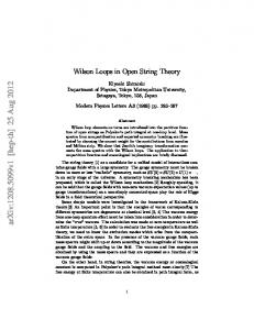
the chosen β–region the non-perturbative parts of the Wilson loops WN M can be well described by an a4 -ansatz with an (a4 )2 correction term. For the difference between the perturbative and the lattice Monte Carlo plaquette ∆W11 this correction is rather small. If infinite or large order perturbation theory was to reflect the long distance properties of QCD, we would expect the Wilson loops to show an arealaw behavior and the static potential to grow linearly with distance. As a result, the Borel transform would exhibit a pole at 1/b0 = 16 π 2 /11, and the coefficients of the perturbative series should show a factorial growth. (Then, for comparison, the gluon condensate would show up as a pole at 2/b0 = 32 π 2 /11.) Instead, we find W (R, T ) ∝
T R
(61)
for R = 2, 3, 4 and T = 5, within a few per cent, and no sign of an infrared renormalon3. This result holds for all couplings within the radius of convergence of the perturbative series, 0 < g 2 . 1.1. In Figure 21 we show the potential difference ∆V DVHR,g 2 L
0.15 0.1 0.05 4
1 3.5 0.8 3
g2
R 2.5
0.6 2
FIG. 21: The perturbative potential difference ∆V obtained from the perturbative Wilson loops up to loop order 20 as function of the distance R and g 2 .
as function of R and g 2 calculated from the series
3
We have nothing to add to [34] and to the argument of [35] that there is no physical significance to these ambiguities.
23 variant of the Creutz ratio ∆V (R) = V (R − 1) − V (R) W (R, T ) W (R − 1, T − 1) (62) = log W (R, T − 1) W (R − 1, T ) using the perturbative Wilson loops up to loop order 20. For a linearly increasing potential one would expect ∆V to be a constant proportional to the string tension. In fact, ∆V decreases with R for all g 2 within the radius of convergence consistent with the expected Coulomb behavior 1/(R(R − 1)). A look at the β function suggests, furthermore, that the perturbative theory is separated from the strong coupling phase through a pole, similar to the supersymmetric Yang-Mills theory [36], indicating that there is no direct contradiction with the strong coupling expansion. A similar result to (61) was found in Monte Carlo simulations of gauge-fixed non-compact lattice QCD [37, 38], which as well take into account small fluctuations of the gauge fields only. This leads us to conclude - on the basis of our present results, nota bene - that the perturbative series carry no information on the confining properties of the theory and the non-trivial features of the QCD vacuum. The positive aspect of this result is that the perturbative tail can be cleanly separated from the Monte Carlo results for the plaquette. Acknowledgements
This investigation has been supported partly by DFG under contract SCHI 422/8-1 and by the EU grant 227431 (Hadron Physics2). R.M. is supported by the Research Executive Agency (REA) of the European Union under Grant Agreement PITNGA-2009-238353 (ITN STRONGnet). We thank the RCNP at Osaka university for providing computer resources. Appendix
We present in Tables A1 - A7 all considered rectangular perturbative Wilson loops of sizes N × M with N, M = 1, . . . , L/2 for different sizes L of the used hypercubic lattices L4 in the form WN M = 1 +
20 X
(n)
WN M g 2n .
(63)
n=1 (n)
The expansion coefficients WN M are the result of the extrapolation to zero Langevin step size using
(17). The reported errors are the fit errors from the extrapolation ε → 0. The presented numbers for larger Wilson loops and higher loop orders are collected irrespective of possible problems with the signal to noise ratio at a given order n as discussed in Section II B and have to be taken with care. In Table A8 we give some perturbative Wilson loops as result of an infinite series using the described hypergeometric model for various β values at L = 12. In Table A9 we collect the values for known loop order coefficients in the infinite volume limit. For W11 the first three loop order coefficients are given in [22, 23] whereas for the larger Wilson loops only the first two loop orders are known [21]. The first order coefficients can be computed to high precision.
24
(n)
n
(n)
W11
(n)
W21
W22
1 −0.332147(22) −0.567064(34) −0.874683(122) 2 −0.033411(15) −0.004571(25)
0.104041(63)
3 −0.013368(13) −0.010094(28)
−0.000735(58)
4
−0.006983(1) −0.006394(13)
−0.002683(12)
5
−0.004179(8)
−0.004167(9)
−0.002284(1)
6
−0.002719(6)
−0.002859(8)
−0.001777(9)
7
−0.001872(6)
−0.002041(8)
−0.001368(1)
8
−0.001342(5)
−0.001503(8)
−0.001063(9)
9
−0.000992(5)
−0.001134(7)
−0.000834(8)
10
−0.000752(4)
−0.000874(6)
−0.000663(7)
11
−0.000581(4)
−0.000684(5)
−0.000534(6)
12
−0.000456(4)
−0.000544(5)
−0.000433(6)
13
−0.000363(3)
−0.000437(4)
−0.000355(6)
14
−0.000292(3)
−0.000355(4)
−0.000293(6)
15
−0.000238(3)
−0.000291(4)
−0.000243(5)
16
−0.000195(2)
−0.000240(4)
−0.000204(5)
17
−0.000161(2)
−0.000200(3)
−0.000171(5)
18
−0.000134(2)
−0.000167(3)
−0.000145(5)
19
−0.000112(2)
−0.000141(3)
−0.000123(4)
20
−0.000094(2)
−0.000119(3)
−0.000105(4)
TABLE A1: Perturbative coefficients for L = 4.
n
(n)
W11
(n)
W21
(n)
W22
(n)
W31
(n)
W32
(n)
W33
1 −0.333112(15) −0.573644(44) −0.907518(112) −0.798086(71) −1.193307(174) −1.500876(291) 2
−0.033829(6) −0.003938(26)
0.118297(96)
3
−0.013641(4)
−0.010199(9)
0.000024(16) −0.002820(12)
0.075949(52)
0.313019(171)
0.609060(335)
4
−0.007202(2)
−0.006571(5)
−0.002375(9)
−0.003622(3)
−0.000139(18)
−0.000273(38)
5
−0.004366(3)
−0.004366(6)
−0.002227(12)
−0.002878(6)
−0.000573(8)
−0.000083(34)
6
−0.002881(4)
−0.003047(7)
−0.001813(12)
−0.002190(8)
−0.000684(1)
−0.000138(7)
7
−0.002014(4)
−0.002214(7)
−0.001440(12)
−0.001675(8)
−0.000629(13)
−0.000147(12)
8
−0.001467(4)
−0.001661(7)
−0.001151(12)
−0.001303(8)
−0.000551(13)
−0.000156(1)
9
−0.001103(4)
−0.001278(6)
−0.000927(1)
−0.001028(7)
−0.000473(1)
−0.000157(8)
10
−0.000850(3)
−0.001004(5)
−0.000755(8)
−0.000824(6)
−0.000404(8)
−0.000150(7)
11
−0.000669(3)
−0.000802(4)
−0.000622(6)
−0.000670(5)
−0.000346(6)
−0.000139(6)
12
−0.000535(3)
−0.000650(3)
−0.000518(4)
−0.000551(4)
−0.000298(4)
−0.000126(5)
13
−0.000434(2)
−0.000533(3)
−0.000435(3)
−0.000458(3)
−0.000257(2)
−0.000114(5)
14
−0.000356(2)
−0.000442(2)
−0.000368(2)
−0.000384(2)
−0.000222(2)
−0.000102(4)
15
−0.000295(2)
−0.000370(2)
−0.000313(2)
−0.000324(2)
−0.000192(2)
−0.000091(4)
16
−0.000247(2)
−0.000312(2)
−0.000268(2)
−0.000276(2)
−0.000167(2)
−0.000080(3)
17
−0.000208(2)
−0.000265(2)
−0.000231(2)
−0.000236(2)
−0.000145(2)
−0.000071(3)
18
−0.000177(2)
−0.000227(2)
−0.000200(2)
−0.000203(2)
−0.000127(2)
−0.000063(2)
19
−0.000151(2)
−0.000195(2)
−0.000173(2)
−0.000175(2)
−0.000111(2)
−0.000056(2)
20
−0.000130(1)
−0.000169(2)
−0.000151(2)
−0.000152(2)
−0.000098(2)
−0.000050(2)
−0.005402(37) −0.050954(108)
TABLE A2: Perturbative coefficients for L = 6.
25
n
(n)
W11
(n)
W21
(n)
W22
(n)
(n)
W31
W41
1 −0.333236(8) −0.574473(16) −0.911469(27) −0.800665(29) −1.023410(49) 2 −0.033852(5)
−0.003818(8)
0.119976(19)
3 −0.013670(3)
−0.010214(4)
0.000196(7)
0.076987(16)
0.206839(26)
4 −0.007229(3)
−0.006594(4)
−0.002321(9)
−0.003628(5)
−0.001501(7)
5 −0.004389(2)
−0.004397(4)
−0.002243(5)
−0.002892(6)
−0.001525(6)
6 −0.002903(2)
−0.003080(3)
−0.001845(5)
−0.002209(5)
−0.001309(6)
7 −0.002034(2)
−0.002246(2)
−0.001478(5)
−0.001697(3)
−0.001076(4)
8 −0.001487(1)
−0.001693(2)
−0.001194(6)
−0.001328(3)
−0.000880(3)
9 −0.001122(1)
−0.001310(2)
−0.000973(7)
−0.001057(3)
−0.000725(3)
10 −0.000869(1)
−0.001035(3)
−0.000800(7)
−0.000854(3)
−0.000601(3)
11 −0.000687(1)
−0.000832(3)
−0.000664(6)
−0.000700(3)
−0.000502(3)
12 −0.000553(1)
−0.000678(3)
−0.000555(6)
−0.000579(3)
−0.000423(3)
13 −0.000451(2)
−0.000560(3)
−0.000468(5)
−0.000484(3)
−0.000358(3)
14 −0.000372(2)
−0.000467(3)
−0.000398(5)
−0.000408(3)
−0.000306(3)
15 −0.000310(2)
−0.000393(3)
−0.000340(5)
−0.000346(3)
−0.000262(3)
16 −0.000261(2)
−0.000333(3)
−0.000292(5)
−0.000296(3)
−0.000226(3)
17 −0.000221(2)
−0.000284(3)
−0.000252(4)
−0.000254(3)
−0.000195(3)
18 −0.000189(1)
−0.000244(2)
−0.000219(4)
−0.000220(3)
−0.000170(3)
19 −0.000162(1)
−0.000211(2)
−0.000191(4)
−0.000191(3)
−0.000148(3)
20 −0.000140(1)
−0.000183(2)
−0.000167(3)
−0.000167(2)
−0.000130(2)
−0.002770(7) −0.002536(14)
TABLE A3: Perturbative coefficients for L = 8.
n
(n)
W32
(n)
W33
(n)
W42
(n)
(n)
W43
W44
1 −1.204201(52) −1.528486(114) −1.485430(97) −1.830535(174) −2.140917(228) 2
0.320661(27)
0.636544(74)
0.595785(62)
1.028662(168)
1.524356(276)
3 −0.005468(14)
−0.055098(20) −0.048959(22)
4 −0.000135(19)
−0.000547(45) −0.000495(31)
0.002744(73)
0.025146(116)
5
−0.000592(1)
−0.000131(15) −0.000219(24)
−0.000108(45)
0.000200(94)
6 −0.000687(12)
−0.000159(28) −0.000216(20)
−0.000068(44)
0.000011(96)
7
−0.000652(1)
−0.000208(13) −0.000238(13)
−0.000082(17)
−0.000067(33)
8
−0.000588(1)
−0.000214(17) −0.000246(11)
−0.000089(14)
−0.000057(28)
−0.174438(58) −0.396169(154)
9
−0.000514(1)
−0.000196(16) −0.000233(11)
−0.000077(15)
−0.000027(26)
10
−0.000443(9)
−0.000174(13)
−0.000209(9)
−0.000063(12)
−0.000011(14)
11
−0.000380(7)
−0.000153(1)
−0.000183(7)
−0.000054(8)
−0.000010(7)
12
−0.000326(6)
−0.000136(8)
−0.000160(6)
−0.000048(7)
−0.000013(5)
13
−0.000281(6)
−0.000120(7)
−0.000141(5)
−0.000043(6)
−0.000015(4)
14
−0.000243(5)
−0.000107(7)
−0.000124(5)
−0.000039(5)
−0.000015(4)
15
−0.000210(5)
−0.000095(6)
−0.000109(5)
−0.000035(5)
−0.000013(4)
16
−0.000183(5)
−0.000084(5)
−0.000096(5)
−0.000032(5)
−0.000011(4)
17
−0.000160(5)
−0.000075(5)
−0.000086(5)
−0.000029(4)
−0.000010(4)
18
−0.000141(4)
−0.000068(4)
−0.000076(4)
−0.000027(4)
−0.000009(3)
19
−0.000124(4)
−0.000061(4)
−0.000068(4)
−0.000025(3)
−0.000008(3)
20
−0.000110(4)
−0.000055(4)
−0.000061(4)
−0.000023(3)
−0.000007(2)
TABLE A4: Perturbative coefficients for L = 8 (continued).
26
n
(n)
W11
(n)
W21
(n)
W22
(n)
W31
(n)
(n)
W41
(n)
W51
W61
1 −0.333320(4) −0.574758(4) −0.912636(19) −0.801260(5) −1.024718(1) −1.247323(13) −1.469522(15) 2 −0.033898(1) −0.003835(2) 3 −0.013698(3) −0.010247(5)
0.120423(2)
0.077139(9) 0.207624(22)
0.387381(18)
0.616194(13)
0.000136(15) −0.002788(4) −0.002610(3)
−0.020698(3) −0.067876(11)
4 −0.007251(3) −0.006625(7) −0.002337(13) −0.003640(8) −0.001503(7)
−0.000967(6) −0.000342(11)
5 −0.004410(3) −0.004425(6) −0.002255(11) −0.002914(9) −0.001539(1)
−0.000784(1)
−0.000475(6)
6 −0.002922(3) −0.003106(6)
−0.001861(9) −0.002233(7) −0.001326(1) −0.000724(12) −0.000406(15)
7 −0.002052(3) −0.002272(4)
−0.001503(7) −0.001726(5) −0.001101(5)
−0.000645(6)
−0.000373(8)
8 −0.001504(2) −0.001718(3)
−0.001217(4) −0.001355(3) −0.000906(3)
−0.000557(4)
−0.000334(6)
9 −0.001138(2) −0.001333(2)
−0.000994(2) −0.001082(2) −0.000748(1)
−0.000475(2)
−0.000289(3)
10 −0.000884(1) −0.001056(2)
−0.000820(2) −0.000876(2) −0.000621(1)
−0.000403(2)
−0.000251(3)
11 −0.000700(1) −0.000851(1)
−0.000683(3) −0.000719(2) −0.000519(2)
−0.000344(2)
−0.000218(3)
12 −0.000565(1) −0.000696(2)
−0.000574(4) −0.000597(3) −0.000438(3)
−0.000295(4)
−0.000191(4)
13 −0.000462(1) −0.000577(2)
−0.000487(4) −0.000502(3) −0.000373(4)
−0.000256(4)
−0.000168(4)
14 −0.000383(1) −0.000484(2)
−0.000418(4) −0.000426(3) −0.000321(4)
−0.000223(4)
−0.000149(3)
15 −0.000320(1) −0.000409(2)
−0.000361(4) −0.000364(3) −0.000278(3)
−0.000196(3)
−0.000132(2)
16 −0.000271(1) −0.000350(2)
−0.000314(3) −0.000315(2) −0.000243(2)
−0.000173(2)
−0.000117(1)
17 −0.000231(1) −0.000301(2)
−0.000275(2) −0.000274(2) −0.000213(2)
−0.000153(2)
−0.000105(1)
18 −0.000199(1) −0.000261(2)
−0.000242(2) −0.000239(2) −0.000188(2)
−0.000136(2)
−0.000094(2)
19 −0.000172(1) −0.000228(1)
−0.000213(3) −0.000210(2) −0.000166(2)
−0.000122(3)
−0.000085(2)
20 −0.000150(1) −0.000200(1)
−0.000189(3) −0.000185(2) −0.000147(3)
−0.000109(3)
−0.000077(2)
TABLE A5: Perturbative coefficients for L = 12.
n
(n)
W32
(n)
W33
(n)
W42
(n)
W43
(n)
(n)
W44
W52
(n)
W53
1 −1.207005(31) −1.535522(52) −1.491384(41) −1.845142(72) −2.170005(100) −2.148586(117) −0.000077(2) 2
0.322694(4)
0.643882(9)
3 −0.005740(18) −0.056823(24)
0.601963(23)
1.048051(37)
1.571598(94)
1.538376(110) −0.000077(2)
−0.050320(9) −0.181032(13)
−0.418636(81)
−0.404144(11) −0.000077(2)
4 −0.000112(19) −0.000446(44) −0.000514(12)
0.003334(36)
0.028597(70)
0.027039(50) −0.000077(2)
5 −0.000592(11) −0.000136(15)
−0.000182(2) −0.000224(12)
−0.000196(13)
−0.000207(18) −0.000077(2)
6
−0.000685(9) −0.000113(15)
−0.000197(8) −0.000059(18)
−0.000019(16)
0.000003(30) −0.000077(2)
7
−0.000663(7) −0.000178(12)
−0.000241(6) −0.000074(13)
−0.000064(18)
−0.000054(20) −0.000077(2)
8
−0.000598(4)
−0.000196(5)
−0.000248(4) −0.000074(11)
−0.000031(14)
−0.000043(20) −0.000077(2) −0.000027(11) −0.000077(2)
9
−0.000523(2)
−0.000192(5)
−0.000234(5)
−0.000067(9)
−0.000024(4)
10
−0.000453(3)
−0.000177(3)
−0.000210(3)
−0.000059(1)
−0.000013(8)
−0.000015(8) −0.000077(2)
11
−0.000391(5)
−0.000161(7)
−0.000188(6)
−0.000056(8)
−0.000015(11)
−0.000018(14) −0.000077(2)
12
−0.000339(6)
−0.000148(9)
−0.000170(7) −0.000058(11)
−0.000023(7)
−0.000025(12) −0.000077(2)
13
−0.000297(6)
−0.000137(9)
−0.000155(7)
−0.000059(8)
−0.000029(5)
−0.000028(7) −0.000077(2)
14
−0.000261(5)
−0.000126(7)
−0.000141(5)
−0.000058(5)
−0.000030(5)
−0.000029(4) −0.000077(2)
15
−0.000230(4)
−0.000116(5)
−0.000128(3)
−0.000055(4)
−0.000026(8)
−0.000026(6) −0.000077(2)
16
−0.000204(3)
−0.000106(5)
−0.000116(3)
−0.000051(6)
−0.000023(11)
−0.000023(8) −0.000077(2)
17
−0.000182(3)
−0.000096(7)
−0.000105(4)
−0.000047(8)
−0.000020(12)
−0.000021(9) −0.000077(2)
18
−0.000162(4)
−0.000087(8)
−0.000095(5)
−0.000043(9)
−0.000018(11)
−0.000020(9) −0.000077(2)
19
−0.000145(5)
−0.000078(9)
−0.000086(6)
−0.000040(9)
−0.000017(9)
−0.000020(8) −0.000077(2)
20
−0.000130(5)
−0.000071(9)
−0.000077(6)
−0.000037(8)
−0.000016(6)
−0.000018(6) −0.000077(2)
TABLE A6: Perturbative coefficients for L = 12 (continued).
27 n
(n)
W54
(n)
W55
(n)
(n)
W62
(n)
W63
(n)
W64
W65
(n)
W66
1 −2.484945(156) −2.807271(225) −2.052506(78) −2.448879(142) −2.794661(184) −3.121967(258) −3.438947(291) 2 3 4 5
2.181680(181)
2.906812(327)
1.391688(52)
−0.790329(77) −1.342663(185) −0.341621(19) 0.101235(36)
0.260769(172)
2.114904(186)
2.879504(270)
3.716609(450)
4.631615(573)
−0.751605(84) −1.322744(141) −2.086833(280) −3.069039(366)
0.020658(33)
0.093854(31)
−0.002457(18) −0.015589(148) −0.000052(25)
−0.002038(23)
0.255213(42)
0.548424(285)
1.025063(600)
−0.015007(49) −0.056854(283) −0.156497(515)
6
0.000160(35)
0.000420(19) −0.000080(18)
0.000078(14)
7
−0.000078(29)
−0.000175(44) −0.000076(11)
−0.000051(12)
−0.000048(49) −0.000388(108) −0.000301(267)
0.000253(48)
0.001978(79)
0.008403(118)
8
−0.000020(16)
−0.000011(8) −0.000059(11)
−0.000045(23)
−0.000034(33)
0.000034(26) −0.000051(119)
9
−0.000008(6)
0.000015(11)
−0.000049(9)
−0.000022(1)
−0.000009(25)
−0.000004(50)
10
0.000007(12)
0.000030(16)
−0.000037(4)
0.000003(1)
0.000015(17)
0.000056(16)
0.000008(124) 0.000093(31)
11
−0.000005(12)
0.000008(1)
−0.000035(3)
0.000002(17)
−0.000004(1)
−0.000014(7)
−0.000066(26)
12
−0.000016(6)
−0.000002(2)
−0.000037(5)
−0.000005(11)
−0.000011(4)
−0.000022(9)
−0.000049(5)
13
−0.000020(4)
−0.000006(1)
−0.000038(3)
−0.000012(5)
−0.000013(11)
−0.000010(9)
−0.000026(17)
14
−0.000019(6)
−0.000008(3)
−0.000038(1)
−0.000016(5)
−0.000009(11)
−0.000004(8)
0.000002(22)
15
−0.000015(8)
−0.000007(6)
−0.000036(2)
−0.000016(5)
−0.000004(9)
−0.000001(7)
0.000012(11)
16
−0.000010(1)
−0.000005(8)
−0.000033(3)
−0.000015(6)
−0.000002(7)
0.000000(6)
0.000014(3)
17
−0.000008(1)
−0.000004(9)
−0.000030(5)
−0.000013(7)
−0.000001(6)
0.000000(5)
0.000009(5)
18
−0.000007(8)
−0.000003(7)
−0.000028(5)
−0.000012(6)
0.000000(5)
−0.000001(4)
0.000002(4)
19
−0.000007(6)
−0.000003(5)
−0.000025(5)
−0.000011(5)
0.000000(3)
−0.000002(3)
−0.000002(3)
20
−0.000006(4)
−0.000002(3)
−0.000023(4)
−0.000010(4)
0.000000(2)
−0.000002(2)
−0.000004(5)
TABLE A7: Perturbative coefficients for L = 12 (continued).
∞ W11
∞ W21
∞ W31
∞ W22
5.85
0.57595(14)
0.36021(22)
0.22936(28)
0.16659(41)
5.9
0.58254(11)
0.36901(16)
0.23814(21)
0.17557(29)
β
5.95 0.588518(92)
0.37692(13)
0.24602(17)
0.18354(24)
0.594092(80)
0.38429(11)
0.25337(14)
0.19095(20)
6.05 0.599358(71)
0.39125(10)
0.26034(12)
0.19797(17)
6.1 0.604372(63) 0.397894(90)
0.26702(11)
0.20469(15)
6.15 0.609172(57) 0.404260(81) 0.273454(99)
0.21118(14)
6.2 0.613784(52) 0.410391(75) 0.279676(89)
0.21745(12)
6.25 0.618228(48) 0.416313(67) 0.285714(81)
0.22355(11)
6.3 0.622521(44) 0.422047(62) 0.291587(74)
0.22949(10)
6
6.35 0.626675(41) 0.427612(57) 0.297310(68) 0.235295(94) 6.4 0.630703(38) 0.433020(53) 0.302895(63) 0.240961(87) 6.45 0.634612(35) 0.438283(49) 0.308354(58) 0.246508(80) 6.5 0.638412(33) 0.443412(45) 0.313694(54) 0.251941(75) 6.55 0.642108(31) 0.448415(44) 0.318922(50) 0.257270(70) 6.6 0.645708(29) 0.453299(40) 0.324046(47) 0.262499(65) 6.65 0.649216(27) 0.458071(37) 0.329071(44) 0.267634(61) 6.7 0.652637(25) 0.462737(35) 0.334001(41) 0.272680(57) 6.75 0.655977(23) 0.467302(33) 0.338842(39) 0.277641(54) 6.8 0.659239(22) 0.471771(31) 0.343596(36) 0.282521(50)
TABLE A8: Summed series of perturbative Wilson loops at L = 12 using the described hypergeometric model as function of β.
28 WN M W11 [22, 23]
(1)
WN M,∞ −1/3
(2)
WN M,∞
(3)
WN M,∞
−0.0339109931(3) −0.0137063(2)
W21 [21]
−0.57483367
−0.003857(17)
W31 [21]
−0.80146372
0.07717(5)
W22 [21]
−0.91287436
0.12040(7)
TABLE A9: Coefficients of lowest loop orders in the infinite volume limit.
29
[1] M. A. Shifman, A. I. Vainshtein and V. I. Zakharov, Nucl. Phys. B 147 (1979) 385. [2] T. Banks, R. Horsley, H. R. Rubinstein and U. Wolff, Nucl. Phys. B 190 (1981) 692. [3] A. Di Giacomo and G. C. Rossi, Phys. Lett B 100 (1981) 481. [4] J. Kripfganz, Phys. Lett. B 101 (1981) 169; R. Kirschner, J. Kripfganz, J. Ranft and A. Schiller, Nucl. Phys. B 210 (1982) 567. [5] E.-M. Ilgenfritz and M. M¨ uller-Preussker, Phys. Lett. B 119 (1982) 395. [6] R. Alfieri, F. Di Renzo, E. Onofri and L. Scorzato, Nucl. Phys. B 578 (2000) 383 [arXiv:hep-lat/0002018]. [7] F. Di Renzo and L. Scorzato, JHEP 0110 (2001) 038 [arXiv:hep-lat/0011067]. [8] P. E. L. Rakow, PoS LAT2005 (2006) 284 [arXiv:hep-lat/0510046]. [9] Y. Meurice, Phys. Rev. D 74 (2006) 096005 [arXiv:hep-lat/0609005]. [10] J. C. LeGuillou and J. Zinn-Justin, Large-Order Behavior of Perturbation Theory, North-Holland, Amsterdam, 1990. [11] S. Narison and V. I. Zakharov, Phys. Lett. B 679 (2009) 355 [arXiv:0906.4312 [hep-ph]]. [12] E.-M. Ilgenfritz, Y. Nakamura, H. Perlt, P. E. L. Rakow, G. Schierholz and A. Schiller, PoS LAT 2009 (2009) 236 [arXiv:0910.2795 [hep-lat]]. [13] R. Horsley, G. Hotzel, E.-M. Ilgenfritz, Y. Nakamura, H. Perlt, P. E. L. Rakow, G. Schierholz and A. Schiller, PoS LATTICE 2010 (2010) 264 [arXiv:1010.4674 [hep-lat]]. [14] G. Parisi and Y. -s. Wu, Sci. Sin. 24 (1981) 483. [15] F. Di Renzo and L. Scorzato, JHEP 0410 (2004) 073 [arXiv:hep-lat/0410010]. [16] G. Bali, private communication. [17] U. M. Heller and F. Karsch, Nucl. Phys. B 251 (1985) 254. [18] R. Horsley, P. E. L. Rakow and G. Schierholz, Nucl. Phys. Proc. Suppl. 106 (2002) 870 [arXiv:hep-lat/0110210]. [19] C. Domb and M. F. Sykes, Proc. R. Soc. A 240 (1957) 214.
[20] G. P. Lepage and P. B. Mackenzie, Phys. Rev. D 48 (1993) 2250 [arXiv:hep-lat/9209022]. [21] R. Wohlert, P. Weisz and W. Wetzel, Nucl. Phys. B 259 (1985) 85. [22] B. Alles, A. Feo and H. Panagopoulos, Phys. Lett. B 426 (1998) 361 [Erratum-ibid. B 553 (2003) 337] [arXiv:hep-lat/9801003]. [23] A. Athenodorou, H. Panagopoulos and A. Tsapalis, Nucl. Phys. Proc. Suppl. 140 (2005) 794 [arXiv:hep-lat/0409127]. [24] F. Di Renzo, G. Marchesini and E. Onofri, Nucl. Phys. B 497 (1997) 435 [arXiv:hep-lat/9612016]. [25] G. Martinelli and C. T. Sachrajda, Nucl. Phys. B 478 (1996) 660 [arXiv:hep-ph/9605336]. [26] See, e.g., M. Beneke, Phys. Rept. 317 (1999) 1 [arXiv:hep-ph/9807443]]. [27] I. M. Suslov, Zh. Eksp. Teor. Fiz. 127 (2005) 1350 [J. Exp. Theor. Phys. 100 (2005) 1188] [arXiv:hep-ph/0510142]. [28] V. Zakharov, Nucl. Phys. Proc. Suppl. 207-208 (2010) 306 [arXiv:1010.4482 [hep-ph]]. [29] E.-M. Ilgenfritz, H. Perlt, A. Schiller, unpublished. [30] G. Burgio, F. Di Renzo, G. Marchesini and E. Onofri, Phys. Lett. B 422 (1998) 219 [arXiv:hep-ph/9706209]. [31] S. Necco and R. Sommer, Nucl. Phys. B 622 (2002) 328 [arXiv:hep-lat/0108008]. [32] M. A. Shifman, Nucl. Phys. B 173 (1980) 13. [33] S. Narison, Phys. Lett. B 387 (1996) 162 [arXiv:hep-ph/9512348]. [34] C. Bauer, G. S. Bali and A. Pineda, Phys. Rev. Lett. 108 (2012) 242002 [arXiv:1111.3946 [hep-ph]]. [35] M. E. Luke, A. V. Manohar and M. J. Savage, Phys. Rev. D 51 (1995) 4924 [arXiv:hep-ph/9407407]. [36] I. I. Kogan and M. A. Shifman, Phys. Rev. Lett. 75 (1995) 2085 [arXiv:hep-th/9504141]. [37] A. Patrascioiu, E. Seiler and I. O. Stamatescu, Phys. Lett. B 107 (1981) 364. [38] E. Seiler, I. O. Stamatescu and D. Zwanziger, Nucl. Phys. B 239 (1984) 177.