Human Dynamics in Large Communication Networks - CiteSeerX

Human Dynamics in Large Communication Networks Christos Faloutsos†

Abstract How often humans communicate with each other? What are the mechanisms that explain how human actions are distributed over time? Here we answer these questions by studying the time interval between calls and SMS messages in an anonymized, large mobile network, with 3.1 million users, over 200 million phone calls and 300 million SMS messages,spanning 70 GigaBytes. Our first contribution is the Truncated Autocatalytic Process (TAP ) model, that explains the time between communication events (ie., times between phone-initiations) for a single individual. The novelty is that the model is ’autocatalytic’, in the sense that the parameters of the model change, depending on the latest inter-event time: long periods of inactivity in the past result in long periods of inactivity in the future, and vice-versa. We show that the TAP model mimics the inter-event times of the users of our dataset extremely well, despite its parsimony and simplicity. Our second contribution is the TAP-classifier , a classification method based on the interevent times and in addition to other features. We showed that the inferred sleep intervals and the reciprocity between outgoing and incoming calls are good features to classify users. Finally, analyze the network effects of each class of users and we found surprising results. Moreover, all of our methods are fast, and scale linearly with the number of customers.

1 Introduction The current availability of large datasets containing digitalized information on human dynamics made it possible for researches to arise questions that many once thought they were already answered: what is the timing of human actions? How often individuals perform a given activity? From several types of datasets, ranging from e-mail records [20, 6] to timestamps from print requests in a student laboratory [12], it was verified that the classic Poisson Process (PP) [11] consistently fails to represent the real data. While in a PP activities occur at a constant rate, the analysis of real data have shown that humans have very long periods of inactivity and also bursts of intense activity [1]. Although modern approaches [1, 16] agree that a PP is not suitable to model human dynamics, a consensus on a final generative mechanism capable of reproducing the observed time intervals between human activities was not yet reached. ∗ Universidade

Federal de Minas Gerais, iLab Mellon University, iLab ‡ Universidade Federal de Minas Gerais

Antonio A.F. Loureiro‡

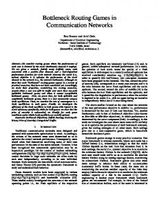
Thus, in this paper, we contribute to this discussion by proposing the Truncated Autocatalytic Process (TAP ). The TAP is a generative model for the time intervals between human activities. Unlike the PP, that is “memoryless”, i.e., the next event arrives independently of the time it took for the previous event to arrive, the TAP model uses a Markovian approach, where the next inter-event time depends on the previous one. In order to validate the TAP model, we examine mobile phone records obtained from the network of a large mobile operator of a large city. More specifically, we analyze the inter-event time between hundreds of million calls and Short Message Service (SMS) messages exchanged between more than three million customers. As we observe in Figure 1, we show that the synthetic data generated by the TAP model strikingly matches the real data. Moreover, it uses only one parameter to model the regular inter-event times: the median of time between activities. We also propose the TAP* model, that is also able to model the time intervals due to sleep periods using only two extra parameters. 4

10 Odds Ratio

Pedro O.S. Vaz de Melo∗

2

10

0

10

real TAP Poisson

−2

10

−4

10

0

10

2

10 ∆t (s)

4

10

Figure 1: The Odds Ratio (defined later - see page 3, Equation 3.2) vs. time interval value between 23217 SMSs of a highly active user of our dataset. Both axes are logarithmic and red, blue and black correspond, respectively, to TAP , real data, and synthetic data generated from a Poisson process. Notice how good is the fit of TAP . For the histogram, see the Appendix. The accurate understanding of the human dynamics can lead to a large variety of applications and to the improvement

† Carnegie

968

Copyright © SIAM. Unauthorized reproduction of this article is prohibited.

of services that already exist. As an immediate application, if we know at what rate humans perform a certain activity in a determined service, e.g. SMS, we also know the rate in which data is generated, what is crucial in the design of the database infrastructure that will support this service. Moreover, once we understand the generative mechanisms behind the time interval between human actions, we may look separately at individuals and quantitatively differentiate them. In this direction, we use the sleep intervals parameters of our proposed TAP model, combined with other aggregate individual features, to classify the users of our dataset in different participation roles. We call this role discovery process the TAP-classifier , which is parameter-free and linear on the number of users. Besides this, we also analyzed the network connections among users from different and equal classes. Amongst others, we discovered that a small portion of the users is responsible for the vast majority of the network traffic and also a surprisingly high number of phone calls between customers that rarely receive phone calls and customers that rarely make calls. In summary, the main contributions of this paper are: • The proposal of the TAP model to generate the interval times between communication activities of individuals; • The TAP-classifier , a parameter-free classification method of mobile phone users that is linear on the number of users; • The network analysis of the customers according to their classifications. The rest of the paper is organized as follows. In Section 2, we provide a brief survey of other work that analyzed individual inter-event times. In Section 3, we describe our proposed TAP model for generating realistic inter-event times and we show its goodness of fit. The TAPclassifier role discovery method and the network analysis is shown in Section 4. Finally, we show the conclusions and future research directions in Section 5.

where U (0, 1) is a uniformly random distributed number between [0, 1]. While in a Poisson process consecutive events follow each other at a relatively regular time, real data shows that humans have very long periods of inactivity and also bursts of intense activity [1]. Modern Approaches To the best of our knowledge, the first modern model for the inter-event times of individuals was the universality class model proposed by Barabási [1]. He proposed that the bursts and heavy-tails in human activity is a consequence of a decision-based queuing process, when tasks are executed according to some perceived priority. In this way, most of the tasks are rapidly executed and some of then may take a very long time. The queuing models proposed in [1] generate power law [8] distributions p(X = x) ≈ x−α with slopes α ≈ 1 or α ≈ 1.5. In the literature, there are examples that are approximated by the universality class model in e-mail records [20, 6], web surfing [20, 5], library visitation, letters correspondence and stock broker’s activity [20], arrival times of requests to print in a student laboratory [12] and in short-messages [21], most of them reporting slopes from 1 to 1.5 and, in the case of [21], also slopes higher than 1.5. In [16], the authors proposed a new approach to model the inter-event times distribution verified in human individuals activity, based on the circadian and weekly cycles and coupled to cascading activity. The model is basically a non homogeneous Poisson with rate λ(t), that depends on time t in a periodic manner. This process generates active intervals accordingly to λ(t). Each active interval initiates a homogeneous Poisson process with a determined rate λa . In order to generate the active intervals, the model needs (i) the average number of active intervals per week and (ii) the probabilities of starting an active interval at a particular time of day and (iii) week. The authors estimated these parameters empirically and they showed that the model accurately fits the real data. They also showed that the universality class model with slope α = 1 proposed in [1] fails to represent the data. Conclusions The fact is that the reports of the universality class model in real data are mostly based on nonrigorous statistical fittings [3], and also fail to reproduce the tasks that take very short inter-event times, that are on the head of the distribution. Moreover, the non homogeneous Poisson Process model proposed by [16] is statistically rigorous but is not parsimonious, depending on several parameters that can only be estimated by empirical data. Therefore, it is clear that there is not yet in the literature a (i) parsimonious and (ii) fully accurate model to describe the inter-event times of human activity. Our goal is to fill this gap with the TAP model.

2 Related work Classic Approach The study of the time interval in which events occur in human activity is not new in the literature. The most primitive model is the classic Poisson process [11]. Although the most recent approaches have among themselves significant differences, they all agree that the timing of human actions systematically deviates from this classical approach. The Poisson process predicts that the time interval ∆t between two consecutive events by the same individual follows a exponential distribution with expected value β and rate λ = 1/β, where 3 TAP Model 3.1 Data Description Before explaining the model, we ∆t = exprnd(β) (2.1) describe the data we use in this work. We analyze mobile = −β × ln(U (0, 1)),

969


phone records of more than 3.1 million customers obtained from the network of a large mobile operator of a large city, with more than 263.6 million phone calls records registered during one month and 376.8 million SMS messages registered during six months. For each phone call, we have information about the duration, the date and time it occurred and encrypted values that represent the source and the destination of the call. We have the same information for the SMS messages, but instead of the duration, we have the time delay it took for a message to leave the source’s mobile phone and arrive at its destination. From now on, we will call the phone records the phone dataset and the SMS records the SMS dataset. We say an communication event occurred at time t when a phone call was made or received in t or when a SMS was sent or received in t. Moreover, we interchangeably call time interval or inter-event time ∆t the time between the occurrence of two communication events. We call the inter-event distribution (IED) the distribution of the set of the time intervals ∆1 , ∆2 , ..., ∆T that occurred between the communication events of a single type, i.e., phone or SMS, for a determined user. In both datasets, since the granularity of t is seconds, all the values of ∆t extracted from them is also in seconds.

tail (head) of the distribution. In order to escape from this drawbacks, we propose the use of the Odds Ratio (OR) function, that is a cumulative function where we can clearly see the distribution behavior either in the head and in the tail. Its formula is given by: (3.2)

OR(x)

=

CDF (x) 1 − CDF (x)

Thus, in Figure 2-b, we plot the OR for the selected user. From the OR plot, we can clearly see that either the exponential and the power law significantly deviates from the real data. Moreover, we can also observe that the OR of the inter-event times seems to follows a power law with a OR slope ρ = 1. In case the selected user is an exception, we evaluated a significant number of different users and the results are consistently the same. This strengthens the controversy on the inter-event time distribution and the need for a more accurate and intuitive model. We begin the presentation of our proposed TAP model by investigating the properties of the Poisson process that, as we have seen in this section and in Section 2, it is not suitable to represent the human dynamics. One of the main characteristics of the PP is that it generates inter-event times in a “memoryless” fashion, i.e., the next event arrives independently of the time it took for the previous event to arrive. Therefore, we investigate in our dataset the time ∆t it takes for an event to arrive when an event arrived after a interval of ∆t−1 . A straight line with slope 0 means that the inter-event times are “memoryless” and, therefore, could be generated by a PP. In Figure 3, we plot, for three typical talkative users, the median of the ∆t s for their respective ∆t−1 s put in logarithmic intervals. The same was done for inter-event times generated from a Poisson process with β = 300 seconds. We observe that, differently from the data generated by the Poisson process that has the “memoryless” property, ∆t has larger values as ∆t−1 grows for these users. This suggests that there is a dependency between the next inter-event time and the previous one. In order to see the generality of this result we show, in Figure 4, the distribution of the Pearson’s correlation coefficient between the ∆t median and the bucketized ∆t−1 for the 100000 more talkative users in our dataset. As we can observe, the vast majority of the users have a strong positive correlation, what means that the next inter-event time is correlated to the previous one. This also corroborates to the fact that the inter-event distribution is not “memoryless” and, therefore, can not be generated by a simple Poisson process.

3.2 Motivation As we mentioned in Section 2, the analysis of large scale real data made it possible to better understand how the inter-event time between activities is distributed and possibly generated. In Figure 2, we show the distribution of the time intervals ∆t for a highly talkative user in our SMS dataset, with 25957 messages sent or received. The histogram is showed in Figure 2-a and, as we can observe, this user had a significantly high number of events separated by small periods of time and also long periods of inactivity. We can also observe a second mode, after the 104 seconds, that represents the sleep intervals of the user, i.e., the time he is probably sleeping and not able to communicate. Moreover, either the power law fitting (PL fitting), that in the best fit has an exponent of − 1.5, and the exponential fitting (EXP fitting), that is generated by a PP, deviates from the real data. Moreover, in finite sparse data that spans for several orders of magnitude, that is the case of IEDs when they are measured in seconds, it is very difficult to visualize the histogram, since the distribution is considerably noisy at its tail. One option is to smooth the data by reducing its magnitude by aggregating data into buckets, with the cost of losing information. Another option is to move away from the histogram and analyze the cumulative distributions, i.e., cumulative density function (CDF) and complementary cumulative density function (CCDF) [3]. These distributions 3.3 The Model In order to explain the human activity beveil the sparsity of the data and also the possible irregularities havior, we propose a dynamic generative process that conthat may occur for any particular reason. However, by using secutive inter-event times are dependent. We call this model the CDF (CCDF) you end up losing the information in the the Truncated Autocatalytic Process (TAP ). As we men-

970


4

∆ (median) (s)

10 count

sleep intervals

10

1

10

t

data power law exponential

1

3

10

2

3

10 10 ∆t (seconds)

2

10

Classic Poisson Process β = 300

4

10

1

3

10

5

Figure 3: The median of the inter-event times ∆t s for their respective preceding ∆t−1 s for three talkative users and for inter-event times generated by the Poisson process, all put in logarithmic intervals.

data power law exponential

0

10

4

sleep intervals slope = 1

10

count

10000

count

Odds Ratio

10

∆t−1 (s)

(a) Histogram

10

5

10

5000

2

10

−5

10

0

10

2

10

4

∆

10

0 −1

t

0

0 correlation

1

(a) Linear scales

(b) Odds Ratio

Figure 2: The inter-event time distribution of a highly talkative user in our SMS dataset, with 25957 sent and received. We observe that either the power law fitting (PL fitting) with exponent 1.5 and the exponential fitting (EXP fitting), generated by a PP, deviates from the real data. We also observe that the OR is very well fitted by a straight line with slope 1. tioned in Equation 2.1, in a PP with expected time interval β, a random event is generated after a time interval ∆t = exprnd(β) = −β ln(U (0, 1)), where U (0, 1) is a uniformly random distributed number between [0, 1]. Since we verified that in real data the inter-event times are not “memoryless”, this classic approach is forbidden and, therefore, there is a dependency between ∆t and ∆t−1 . Thus, the TAP model considers that

10 −1

0 correlation

1

(b) Logarithmic scales

Figure 4: The distribution of the correlations between the ∆t median and the bucketized ∆t−1 for the 100000 more talkative users in our dataset. The vast majority of the users have a strong positive correlation, what means that the next inter-event time is correlated to the previous one. the TAP , the inter-event time ∆t between the current event and the next one is given by (3.4)

∆t

= =

exprnd(∆t−1 + C) −(∆t−1 + C) ln(U (0, 1))

where C > 0 is the location parameter that has to be higher than 0 to avoid ∆t to converge to 0 (see more details on the Appendix). In summary, the TAP states that the expected inter-event time ∆t is generated by a classic PP with expected value β = ∆t−1 + C. In Figure 5-a, we plot the histogram of 100000 time intervals ∆t generated by the TAP model with C = 1. (3.3) ∆t = f (∆t−1 ) Moreover, in Figure 5-b, we plot the OR for the same where f is a function that describes the dependency between time intervals. While a classic PP generates a exponential ∆t and ∆t−1 . distribution, we observe that the generated data by the TAP We propose that the expected inter-event time β of the perfectly fits a log-logistic distribution [9] with the OR slope classic Poisson process is dynamic and dependent on the ρ = 1, exactly like the real data shown in Figure 2-b. previous time interval, as described in Equation 3.3. Thus, in Moreover, the tail of the distribution in Figure 5-a is similar

971


Odds Ratio

5

0

µ

Odds Ratio

count

to a power law with slope 2, that is close to what was reported of C = 1. Thus, in Figure 6-a, we plot the OR for different in the literature and discussed in Section 2. The TAP model values of C. As we can observe, changing the value of C changes µ and, consequently, the location of the distribution, is fully described in Algorithm 1. but maintains its shape, since they are parallel. In order to investigate the relationship between C and µ, Algorithm 1: TAP we run 33 simulations of the model for all integer values of C input : n, C > 0 between [1,10000]. As we observe in Figure 6-b, the median output: inter-event times ∆t of the distribution µ varies linearly with C according to a 1 ∆1 ← C; slope of 2.72, that can be approximated by Euler’s number 2 for t ← 2 to n do e, in a way that 3 ∆t ← ceil(exprnd(∆t−1 + C)); (3.5) µ = e × C, 4 end that allow us to generate inter-event times with a determined µ. We ignore the constant factor 3.8 because its 95% confidence interval is (−8.596, 16.3), which contains zero. 10 10 Nevertheless, in order to generate more realistic data, we data fitting 2 should also be able to generate the sleep intervals verified in 10 0 Figure 2. We expect that a talkative user that had a communi10 1 data 10 cation activity in d consecutive days will have as his d highfitting est inter-event times his sleep intervals. Then, we collected −10 0 10 −5 10 −5 0 5 0 5 the d highest inter-event times for several talkative users and 10 10 10 10 10 10 ∆t ∆ t we verified, by performing the Kolmogorov-Smirnov goodness of fit (KS) test, that they all follow a log-logistic distri(a) Histogram (b) OR bution with parameters µs and ρs . Therefore, we can genFigure 5: Inter-event times ∆t generated by the TAP . erate sleep intervals by simply changing the d highest interThe generated ∆t s are perfectly fitted by a log-logistic event times generated by the TAP model to random numbers generated by a log-logistic distribution with parameters µs distribution with the slope ρ = σ = 1. and ρs . The log-logistic distribution was first proposed by 4 x 10 10 Fisk [9] to model income distribution, after observing that 3 C = 10 synthetic data C = 300 the OR plot of real data in log-log scales follows a power µ = 2.7 × C + 3.8 C = 50000 ρ 2 law OR(x) = cx . In summary, a random variable is log10 logistically distributed if the logarithm of the random vari1 able is logistically distributed. The logistic distribution is very similar to the normal distribution, but it has heavier 10 0 10 10 10 10 0 5000 10000 ∆t tails. In the literature, there are examples of the use of the C log-logistic distribution in survival analysis [2, 15], distribu(a) OR for three different values of (b) µ as a function of C tion of wealth [9], flood frequency analysis [17], software reC liability [10] and phone calls duration [4]. From now on, we will characterize a log-logistic distribution by the OR power Figure 6: Changing the value of C changes the location law slope parameter ρ and by the median of the distribution of the distribution. The median of the distribution µ varies µ, i.e., OR(µ) = 1. A commonly used log-logistic parame- linearly with C, µ = a × C + b, with a = 2.6 and b = 3.8. terization considers the parameters ln(µ) and σ = 1/ρ [13]. The 95% confidence interval for a is (2.715, 2.723) and for b Moreover, when σ = 1, it is the same distribution as the Gen- is (−8.60, 16.3). Since the confidence interval for b contains eralized Pareto distribution [14] with shape parameter κ = 1, 0, b is not significative. scale parameter µ and threshold parameter θ = 0. The complete model, that we call TAP* , is described 3.4 Model Parameterization After defining the basic in Algorithm 2. The function llgfit and llgrnd give, respecevent generation mechanism as the TAP model, we can adapt tively, the best fit and the random number generator for the it so it is able to fully mimic the realistic inter-event times log-logistic distribution. The ceil function is a function that data. The first point we consider is the median µ of the inter- rounds up every non-integer number to the lowest integer event times generated by the TAP model. As we mentioned, number that is higher than it. We use the ceil function bewhen OR(x) = 1, x is the median µ of the distribution. We cause the granularity of our data is in seconds and, therefore, see in Figure 3-b that µ is close but different than the value all fractional intervals should be rounded up. −5

−5

972

0

5

10


distribution. In Figure 8, we show the distribution of the empirical slope ρi for the users i of the phone dataset. In this histogram of Figure 8-a we observe that the mode is near ρi = 1. Moreover, in Figure 8-b, we plot the isocontours of ρi and ci , when darker colors mean a higher concentration of pairs ρi and ci and white color mean that there are no users with these values of ρi and ci . We observe that exists a small correlation between ρi and ci , but ρi is consistently around 1.

Algorithm 2: TAP* input : n, µ > 0, d, µs , ρs output: inter-event times ∆t

4 5 6 7 8 9 10 11

4

12

x 10

# of phone calls

3

∆1 ← µ; for t ← 2 to n do //AUTO CATALYTIC STEP; ∆t ← ceil(exprnd(∆t−1 + µ/e)); end //HANDLING SLEEP INTERVALS; //sort to get the d highest ∆t s; ∆t ← sort(∆t ); for s ← n − d + 1 to n do ∆st ← llgrnd(µs , ρs ); end

10 8 count

1 2

6 4

3

10

2

10

2 0 0

We would like to emphasize that, since the slopes of the users of our datasets are, in general, close to 1, we do not create an extra parameter to deal with the slope of the OR of the IED generated by TAP . Thus, the TAP model always generate IED with a OR slope ρ ≈ 1. We also point out that the choice of ∆1 does not change the final result, considering that n is high. We set ∆1 as µ because µ is the inter-event value that evenly separates in the distribution the inter-event times that characterize bursts of activities and the inter-event times that characterize the long periods of inactivity.

Figure 8: Distribution of the empirical slope ρi for the users i of the phone dataset. In (a) we show the histogram of the slope ρi for users that had more than 120 phone calls ci made or received. Observe that the mode is near ρi = 1. Moreover, observe in (b) that exists a small correlation between ρi and ci , but ρi is consistently around 1.

3.5 Validation In this section we look at the inter-event times ∆t of the individuals of both our datasets. In Figure 7, we plot the OR of the inter-event times ∆t for three highly talkative users of the phone dataset. Moreover, we generated synthetic inter-event times using our model TAP* described in Algorithm 2 and also using the Poisson process. As we can observe, the synthetic data generated by the TAP* model mimics almost perfectly the real data, that is mostly a straight line on the log-log scales. The tail of the distribution is marked by the sleep intervals and, once again, the model could reproduce the real data very well. The only difference between the distributions is the initial part, that in the real data does not contain ∆t values lower than some value ∆s ≈ 10. This is explained by the fact that the time between two consecutive calls is lower bounded by a setup time ∆0t that involves dialing the numbers, waiting for the signal, waiting for the other part to answer and so on. We point out that ∆0t could be easily inserted as a parameter in our model but our intent is to leave the TAP* model as general as it is possible. As expected, the synthetic data generated by the PP fail to reproduce the real data. We continue our validation by performing the KS test for the log-logistic distribution on the inter-event times of all individuals of our dataset. We report that more than 96% of the users’ IEDs can statistically be fitted by a log-logistic

Moreover, in Figure 9, we plot the OR of the interevent times ∆t for three highly talkative users of the SMS dataset. We again generated synthetic inter-event times using our TAP* model and the Poisson process. As we can observe, the synthetic data generated by the TAP* model mimics almost perfectly the real data. Moreover, we observe that the head of the distribution of the real data is also fitted considerably well. This happens because when a user sends a message to multiple recipients, the inter-event time between each message tends to be zero or near zero. Besides this, companies provide SMS services in which a robot automatically responds to a SMS message, replying almost immediately another SMS. This, of course, generates records with very small inter-event times. Finally, we also observe that the tail of the distribution is again marked by the sleep intervals, that were correctly reproduced by the synthetic data. Once again, the synthetic data generated by the PP fail to reproduce the real data. Unfortunately, the global analysis of the SMS users, like we did for the phone users, is jeopardized by the existence of a significative transmission delay for a large fraction of the messages. This transmission delay is the time between a message leaving a mobile phone and arriving at the destination. It may happen, for instance, due to infrastructure or personal issues, e.g., a customer left his

973

1

slope ρ

2

(a) Histogram

3

0.5

1 2 slope ρ

(b) Isocontours


Odds Ratio

Odds Ratio

0

real TAP Poisson

2

10

−2

10

0

10

−2

0

10

2

10

4

∆ (s)

0

10

10

0

10

−2

10

10

10

real TAP Poisson

2

Odds Ratio

real TAP Poisson

2

10

10

t

2

10 ∆ (s)

4

0

10

10

t

(a) 910 calls

2

4

10 ∆ (s)

10

t

(b) 1210 calls

(c) 1840 calls

Figure 7: OR for the IEDs of three highly talkative users in the phone dataset and their respective synthetic data generated by either the TAP* model and by a Poisson process. 4

10

2

10

0

10

real TAP Poisson

−2

10

−4

10

0

10

2

10 ∆ (s) t

(a) 23217 messages

4

10

2

10

0

10

real TAP Poisson

−2

10

−4

10

0

10

2

10 ∆ (s) t

(b) 25957 messages

4

10

Odds Ratio

10 Odds Ratio

Odds Ratio

4

4

10

2

10

0

10

real TAP Poisson

−2

10

−4

10

0

10

2

10 ∆ (s)

4

10

t

(c) 17819 messages

Figure 9: OR for the IEDs of three highly communicative users in the SMS dataset and their respective synthetic data generated by the TAP* model. mobile phone unattended and the battery died, delaying all the incoming SMS messages for when the mobile phone is recharged again. These delays overestimate the interevent times between SMS messages, making the majority of the IEDsignificantly noisy. However, for highly talkative users, like the ones in Figure 9, the delays are less frequent and, therefore, do not play a significative role, making their IEDs to be accurately represented by the TAP* model. We report that more than 10% of the users of our dataset can be accurately represented by the TAP model. Moreover, for an intuitive modification of the TAP model that explains the noisy IEDs in the SMS dataset using random transmission delays, see the Appendix. 4 Applications In this section, we show a possible applicability of the TAP model, combining the knowledge acquired in the previous section together with other individual features of the customers of our phone dataset. Firstly, we classify them into different participation roles and, secondly, we use this classification to understand how the classes call each other. In Section 4.1 we show a parameter-free classification method and, in Section 4.2, we show the network behavior of each

974

class. We do not use the SMS dataset because, as we mentioned in the previous section, it is significantly noisy concerning its timestamps records. 4.1 Classes The first individual feature we investigate is the number of phone calls ci a user i sent or received. In Figure 10, we show the distribution of ci for the users i of our phone dataset. We observe that the distribution has, initially, a smooth decay, than a region that is almost uniform and, finally, a strong super linear decay. Thus, we define the users i that have a ci value lower than the point of local maxima situated in the beginning of the super linear decay as the occasional users class. Specifically, the point of local maxima is ci = 94. Since we have temporal data, we believe that it is also interesting to differentiate users that were consistently active in the network from users that had a bursty behavior, i.e., that were active for only a period of the month. If we separate these users, we can accurately characterize the constantly active users according to their regular and sleep inter-event times, that can be captured by the TAP* model. Thus, we define the intermittent class as the class that contains all the users that have talked on at most 75% of


4

count

10

3

10

2

point of local maxima

1

occasional talkatives

10 10

0

10 0 10

2

10 # of phone calls

4

10

Figure 10: Histogram of the number of calls ci per user. The point of local maxima (ci = 94) defines the threshold for characterizing a customer as talkative or occasional. the days of the month, which represents less than 10% of the non-occasional users. We define this threshold as 75% to guarantee that the sleep intervals of the non-intermittent users contain actual sleep intervals. If, for instance, we do not separate these users, a user i with ci = 100 that talked only in the first day of the month would have, according to Algorithm 2, a sleep interval median equal to his regular inter-event time median. Thus, in Figure 11 we show the histogram of the regular inter-event times median µ and sleep intervals median µs of the non-intermittent users. As we observe, there is a clear “gap point” on both histograms, marking two different behaviors. In Figure 11-a, the gap point defines the threshold for the user class call center , that is characterized for mobile phone numbers that are regularly active, since the gap point, in this case, is at µ = 120 seconds. On the other hand, in Figure 11-b, the gap point defines the threshold for the users that are part of the class insomniac , that features mobile phone numbers that are active during the whole day, i.e., that do not sleep. The gap point is, in this case, at µs = 5 hours. It is important to point out that the intersection between the set of users that belong to the call center class and to the insomniac class is the empty set ∅.

count

call center 4

gap point

10 count

4

10

2

10

0

10 0 10

2

4

10 10 ∆t median (s)

(a) regular intervals

gap point

occasional , intermittent , call center or insomniac are, in summary, customers that are constantly active during the whole month and also have human-like behavior in their regular and sleep interval times. Thus, in order to classify them, we make use of another individual feature, that we call reciprocity. Given a user i, with cout outgoing calls i and cin incoming calls, we define the reciprocity ri = i in (cout + 1)/(c + 1). Thus, users with r ≈ 1 are users i i i in that made a similar number of cout and c calls, coherent i i with human behavior. Moreover, users with ri ≫ 1 have cout significantly higher than cin i i , making him a probable “spammer” or telemarketer and, finally, users with ri ≪ 1 have cout significantly lower than cin i i , a common behavior of public service numbers or restaurant deliveries, for instance. Thus, in Figure 12, we plot the isocontours of the logarithms of the reciprocity ri and the sleep intervals medians µsi of the remaining non-classified users i of our phone dataset. We clearly observe three distinct clusters of users, one with low values of ri , one with ri ≈ 1 and other with high values of ri . Given the clear distinction, we run the clustering algorithm k-means [18] with k = 3 and, as expected, the resulting centroids were compatible with the results in Figure 12. Each cluster defines, then, the remaining classes of our role discovery process. The first class is represented by the resulting centroid a(µsi = 12.8h, ri = 0.85), that from now on we call the regular users. The resulting centroid b(µsi = 14.0h, ri = 0.06) is the one that defines the class 9-5 business , while the resulting centroid c(µsi = 12.0h, ri = 19.4) defines the class spammer .

sleep interval median (h)

5

10

b a

1

10

−2

10

c

0

2

10 10 reciprocity

2

10

Figure 12: Isocontours of the reciprocity ri and the sleep interval median of the users in our dataset. Observe the clusters marked by circles: (a) regular , (b) 9-5 business and (c) spammer .

insomniacs

0

10 0 10

1

2

10 10 sleep interval median (h)

(b) sleep intervals

Figure 11: The gap points define the threshold for characterBesides the obvious discrepancies concerning the ri , the izing the classes 9-5 business and insomniac . subtle differences among the centroids’ µsi are coherent with the classes definitions. The higher value of µsi for the 9The remaining customers that were not characterized as 5 business class probably means that the phone numbers of

975


these users are mostly and, sometimes only, active during O BSERVATION 1. Although the majority of users are occabusiness hours. On the other hand, the lower values of µsi sional users (62%), most of the calls (88%) are directed to for the spammer class indicates that the calls are also made regular and call center phone numbers. when the regular users are already at home, being able to Observation 1 arises an interesting scenario that mobile calmly talk. The full TAP-classifier mechanism is described phone companies have to deal with: the vast majority of their in Figure 13. network traffic is caused by a small fraction of their clients. This is probably due to the fact that most of the mobile companies offer unlimited mobile plans that impose no extra # OF CALLS < POINT OF LOCAL costs for their subscribers, enabling them to make phone OCCASIONAL Y MAXIMA (94) calls whenever they want, for the weakest of the reasons. N On the other hand, companies also offer pre-paid plans, that TALKED IN LESS demand no contracts and usually cheaper to acquire, but at THAN 75% OF Y INTERMITTENT THE DAYS the cost of a more expensive price per phone call made and, sometimes, received. Users of this type of plan tend to only N use the phone when it is really necessary. Moreover, the observed proportion of occasional users per regular users CALL CENTER INTER-EVENT TIME Y MEDIAN < GAP can be explained by the fact that monetary and bureaucratic POINT (2 MINUTES) effort to acquire a pre-paid phone is considerably smaller N than the effort to subscribe to an unlimited plan, what makes SLEEP INTERVAL MEDIAN < GAP the pre-paid phones really attractive for users that do not POINT (5 HOURS) Y INSOMNIAC need to use mobile phones actively. N REGULAR

−50%

9-5 BUSINESS

0%

+50% occasional intermittent call center insomniacs regular 5−7 business spammer

SPAMMER

976

ca

in

oc

4.2 Network Effects Since the classes are defined, we are now able to verify how nodes from determined classes communicate with each other. In this section, we only consider calls that were made between clients of the mobile phone operator of our dataset. In Table 2 we list the number c(ri , rj ) and the percentage p(ri , rj ) of phone calls made from the users of the “row” class ri to the users of the “column” class rj . For instance, 5% of the calls made from the users that belong to the occasional class are directed to the users that belong to the intermittent class, a total of 80563 phone calls. Moreover, in Figure 14 we show the colormap of the differences between p(ri , rj ) and the percentages pRN D (ri , rj ) resulting from the random Erdös-Rényi (ER) model [7], that, in this case, generates a random call graph with the same number of vertices, edges and outgoing calls. Red colors mean negative differences, blue colors mean positive differences and green colors mean small differences. In other words, if the color between class ri and class rj is red, then ri avoids class rj , if it is green, they talk at random and, if it is blue, class rj attracts phone calls from users of class ri .

si on a te rm l itt ca ent ll ce n in so ter m ni ac s re 5− gu 7 l bu ar si ne ss sp am m er

Figure 13: The TAP-classifier mechanism.

caller class

K-MEANS USING SLEEP INTERVALS AND RECIPROCITY

callee class

Figure 14: Heatmap of the difference between the percentages on Table 2 and the percentages generated randomly. Red colors mean negative differences, blue colors mean positive differences and green colors mean small differences. The darker the color, the bigger the difference.

O BSERVATION 2. Customers that rarely make phone calls, i.e., 9-5 business , are more likely to receive calls from customers that rarely receive calls, i.e., spammer . Although 9-5 business users still receive, in general, most of the calls originated from regular users, the fraction of calls originated from spammer users is very significative when comparing with the proportion the other classes receive


Table 1: Customer classes. Class Label occasional intermittent call center insomniac regular 9-5 business spammer

Summary Users that have made or received few phone calls Users that have talked in less that 75% of the days Phones that are constantly active during the day Users that do not have sleep intervals Regular active users Users that rarely make phone calls Users that rarely receive phone calls

# of users 1914645 110795 348 361 748109 250773 87756

% 61% 4% 0.01% 0.01% 24% 8% 3%

Table 2: Number of calls between users. Caller/Callee occasional intermittent call center insomniac regular 9-5 business spammer Total

occasional 299207 (19%) 368309 (9%) 754 (5%) 766 (5%) 3953380 (6%) 153851 (9%) 896253 (8%) 5672520 (6%)

intermittent 80563 (5%) 368309 (10%) 721 (5%) 585 (4%) 3230513 (5%) 75466 (4%) 552580 (5%) 4329486 (5%)

call center 264 (0.02%) 468 (0.01%) 0 (0%) 11 (0.01%) 10893 (0.01%) 348 (0.02%) 1538 (0.01%) 13522 (0.01%)

insomniac 265 (0.02%) 580 (0.01%) 0 (0%) 0 (0%) 10765 (0.01%) 176 (0.01%) 1393 (0.01%) 13179 (0.01%)

from them. This surprising observation shows a strong connection between two classes that are complementary and opposite. A possible and reasonable scenario in which this may happen is, for instance, when a central controller of a determined company distributes its services to its employees using a particular mobile phone. This mobile phone almost exclusively make phone calls, which characterize it as a spammer . On the other hand, the employees also almost exclusively use their phones to receive requests of services, what characterize them as 9-5 business . This explanation is also coherent with the sleep intervals of these classes. While most of the employees do not receive requests outside business hours, the central controller may make a few extra phone calls to employees that decided to work for extrahours. We suggest that filtering the spammer and 9-5 business users that have most of the calls among themselves might bring an extra class for the TAP-classifier . We leave this to future work. O BSERVATION 3. At least 23% of the phone calls are nonpersonal phone calls. Observation 3 comes from the fact that 23% of the phone calls are directed to 9-5 business users, that rarely make phone calls. Thus, in this case, since the caller had probably not received before a call from the 9-5 business number he called and is also not expecting to receive in the future, we strongly believe that the vast majority of phone calls directed to 9-5 business phone numbers are non-personal phone calls. These calls are probably service requests calls, in which the caller wants some service to be done from the responsable of the 9-5 business phone number he is calling, that might be a pizza delivery center, a technical support number or the mobile phone of a taxi driver.

977

regular 910613 (57%) 2337923 (60%) 9362 (63%) 10638 (73%) 47870777 (68%) 1076787 (63%) 6117391 (52%) 58333491 (65%)

9-5 business 301920 (19%) 763513 (20%) 3836 (26%) 2508 (17%) 15062387 (21%) 367005 (21%) 4043566 (34%) 20544735 (23%)

spammer 18979 (1%) 46219 (1%) 104 (0.7%) 167 (1%) 688646 (1%) 46998 (3%) 225872 (2%) 1026985 (1%)

Total 1611811 (2%) 3906070 (4%) 14777 (0.02%) 14675 (0.02%) 70827361 (79%) 1720631 (2%) 11838593 (13%) 89933918

Besides these observations, we also point out that either the occasional and the intermittent users are more likely to talk to themselves (see the two first cells from the main diagonal of Table 2 or Figure 14) than the other classes do. This indicates that users of these classes are also more likely to have friends that belong to these classes than the other classes do, which suggests a low degree of homophily, e.g., people that acquire pre-paid phones are more likely to have friends with pre-paid phones than users that subscribe to the more expensive unlimited plans. Moreover, concerning call center and insomniac users, they differ approximately in 10% of their phone calls. While the first ones call 10% more 9-5 business users, what is consistent with its name and definition, the insomniac users call 10% more regular users, what suggests that insomniac may be doctors or other professional that might require a constant vigilance. 5 Conclusions In this paper, we explored the human dynamics of the users of a large mobile company of a large city. We analyzed more than 3 million customers and 200 million phone calls recorded during one month and 370 million SMS messages recorded during six months, making a total of 70 GB of data. This work was mainly motivated by the lack of consensus between the existing models that explain the time interval between human activities. An accurate and parsimonious model for the human dynamics can lead to a large variety of applications and to the improvement of a vast number of services that already exist. The main contributions of the paper can be summarized as follows: • Proposal of TAP model, that matches real data well, and has a very simple, intuitive explanation: the time for the next communication event depends on the time it took


for the previous event to occur;

6.2 The need for C in TAP

Count

• Proposal of TAP-classifier , a parameter-free classification mechanism for customers of mobile phone net- L EMMA 6.1. The constant C > 0 of Equation 3.4 is needed to assure that the inter-event times generated by the TAP works, that is linear on the number of customers; model will not converge to zero. • Analysis of the communication network effects from the classification perspective that, amongst other things, may be applied to anomaly detection and link prediction Proof. If we remove the constant C from Equation 3.4, algorithms. ∆t = −∆t−1 × ln(U (0, 1)). The probability of generating a ∆t value lower than ∆t−1 is P (− ln(U (0, 1)) < 1) = 0.63. As future work, we aim to investigate the foundations Thus, the expected ∆t when t → ∞ is 0. With C in the of the TAP model in order to answer the main question this equation, even when ∆t−1 = 0, ∆t = −C × ln(U (0, 1), paper raised: why either the generated data from the TAP that is a classic Poisson process with β = C and obviously model and real data show a truncated log-logistic inter-event does not converge to 0. time distribution with slope ρ = 1? We plan to analyze other datasets that have individual timestamps records and 6.3 Delay in the SMS dataset In Figure 16-a, we plot the verify whether we can state it is a new theorem. Moreover, a histogram of the SMS transmission delays, that is the time second promising direction is to verify whether a community between a message leaving a mobile phone and arriving at identification framework [19] can aid in our classification the destination. We observe the existence of a significative and network analysis process. In the same direction, it would transmission delay for a large fraction of the messages. be interesting to use, instead outgoing and incoming calls, Since the delay is significative, the inter-event times have measures of relationship strength [22] in the TAP-classifier embedded in themselves the actual human delay and other and verify if the network analysis results change. noisy non-regular delays caused by the mobile network infrastructure or personal issues, e.g., a customer left his 6 Appendix mobile phone unattended and the battery died, delaying all 6.1 The histogram of the TAP model As we observe in the incoming SMS messages for when the mobile phone is Figure 15, the histogram of the inter-event times generated recharged again. Imagine, for instance, that Smith had sent a by the TAP model also fits very well the real data. As message to John at time t1 and, due to a transmission delay we have seen, the Poisson process forbids the generation of d1 , the message arrived only at t2 . In his turn, Smith saw inter-event times significantly higher than the median of the the message at t2 and immediately replied, but again, due to a transmission delay d2 , the message arrived to John only distribution. at t3 . Thus, for John, the inter-event time between sending 4 the message and receiving the reply is ∆t = t3 − t1 = 10 (t2 +d2 )−(t1 +d1 ), with two transmission delays embedded real in the registered inter-event time. TAP Based on this, we investigate how our TAP model would Poisson behave when we add random delays to the generated inter2 10 event times. The random delays are extracted from the empirical distribution fd showed in Figure 16-a. Since we do not know how many delay times nd are embedded, we define that nd = round(exprnd(2)). Given our Smith and John 0 example, we believe that 2 is a good estimate on the average 10 0 2 4 number of delays to be added in a inter-event time. We use 10 10 10 the exponential distribution (exprnd) because, despite of the ∆t (30s) fact that the average is 2, some inter-event times may have no delay between them, e.g. two consecutive sent messages, Figure 15: The histogram of the time interval values between or, sporadically, several delay times, e.g., when a group of the 23217 SMSs of the same user of Figure 1. Both axes are people is scheduling an event using circular messages. As logarithmic and red, blue and black correspond, respectively, we observe in Figure 16-b, the synthetic data generated by to TAP , real data, and synthetic data generated from a this modified version of the TAP model can fairly reproduce Poisson process. Notice how good is the fit of TAP even the noisy real data, that is the IEDfor a typical customer in when we see the histogram. our SMS dataset. This shows that the transmission delays play an important role in the IEDs of our SMS dataset.

978


6

5

10

10

real synthetic Odds Ratio

count

4

10

2

10

0

10 0 10

0

10

−5

2

4

10 10 delay (5 minutes)

(a) Delay distribution.

10

0

10

2

10

4

∆t

10

6

10

(b) Adding random delay times to the TAP model generated data.

Figure 16: In (a) the distribution of the delay time between a message leaving a mobile phone and arriving at the destination. In (b), we add random delay times using the distribution in (a) to the TAP model. The synthetic data can fairly reproduce the real data, that is the inter-event times of a typical user of our SMS dataset. Acknowledgments. We thank the Conselho Nacional de Desenvolvimento Cient´ıfico e Tecnológico (CNPq) for financial support. Research was also sponsored by the Army Research Laboratory and was accomplished under Cooperative Agreement Number W911NF-09-2-0053. The views and conclusions contained in this document are those of the authors and should not be interpreted as representing the official policies, either expressed or implied, of the Army Research Laboratory or the U.S. Government. The U.S. Government is authorized to reproduce and distribute reprints for Government purposes notwithstanding any copyright notation here on. References [1] A.-L. Barabási. The origin of bursts and heavy tails in human dynamics. Nature, 435:207–211, May 2005. [2] Steve Bennett. Log-logistic regression models for survival data. Journal of the Royal Statistical Society. Series C (Applied Statistics), 32(2):165–171, 1983. [3] Aaron Clauset, Cosma R. Shalizi, and M. E. J. Newman. Power-law distributions in empirical data. SIAM Review, 51(4):661+, Feb 2009. [4] Z. Dezsö, E. Almaas, A. Lukács, B. Rácz, I. Szakadát, and A.-L. Barabási. Dynamics of information access on the web. Physical Review E (Statistical, Nonlinear, and Soft Matter Physics), 73(6):066132, 2006. [5] Jean-Pierre Eckmann, Elisha Moses, and Danilo Sergi. Entropy of dialogues creates coherent structures in e-mail traffic. Proceedings of the National Academy of Sciences of the United States of America, 101(40):14333–14337, October 2004. [6] P. Erdös and A. Rényi. On the evolution of random graphs. Publ. Math. Inst. Hung. Acad. Sci., 7:17, 1960. [7] Michalis Faloutsos, Petros Faloutsos, and Christos Faloutsos. On power-law relationships of the internet topology. In SIGCOMM, pages 251–262, 1999.

979

[8] Peter R. Fisk. The graduation of income distributions. Econometrica, 29(2):171–185, 1961. [9] Swapna S. Gokhale and Kishor S. Trivedi. Log-logistic software reliability growth model. In HASE ’98: The 3rd IEEE International Symposium on High-Assurance Systems Engineering, pages 34–41, Washington, DC, USA, 1998. IEEE Computer Society. [10] Frank A. Haight. Handbook of the Poisson distribution [by] Frank A. Haight. Wiley New York,, 1967. [11] Uli Harder and Maya Paczuski. Correlated dynamics in human printing behaviour. Physica A, 361(1):329–336, 2006. [12] J. F. Lawless and Jerald F. Lawless. Statistical Models and Methods for Lifetime Data (Wiley Series in Probability & Mathematical Statistics). John Wiley & Sons, January 1982. [13] M. O. Lorenz. Methods of measuring the concentration of wealth. Publications of the American Statistical Association, 9:209–219, 1905. [14] Talat Mahmood. Survival of newly founded businesses: A log-logistic model approach. JournalSmall Business Economics, 14(3):223–237, 2000. [15] R. Dean Malmgren, Daniel B. Stouffer, Adilson E. Motter, and Lu´ıs A. N. Amaral. A poissonian explanation for heavy tails in e-mail communication. Proceedings of the National Academy of Sciences, 105(47):18153–18158, November 2008. [16] C.D. Sinclair M.I. Ahmad and A. Werritty. Log-logistic flood frequency analysis. Journal of Hydrology, 98:205–224, 1988. [17] G.A.F. Seber. Multivariate Observations. Wiley, New York, 1984. [18] Chayant Tantipathananandh, Tanya Berger-Wolf, and David Kempe. A framework for community identification in dynamic social networks. In KDD ’07: Proceedings of the 13th ACM SIGKDD international conference on Knowledge discovery and data mining, pages 717–726, New York, NY, USA, 2007. ACM. [19] Pedro O. S. Vaz de Melo, Leman Akoglu, Christos Faloutsos, and Antonio Alfredo Ferreira Loureiro. Surprising patterns for the call duration distribution of mobile phone users. In ECML/PKDD (3), volume 6323 of Lecture Notes in Computer Science, pages 354–369. Springer, 2010. [20] Alexei Vazquez, Joao Gama Oliveira, Zoltan Dezso, KwangIl Goh, Imre Kondor, and Albert-Lazlo Barabasi. Modeling bursts and heavy tails in human dynamics. Phys Rev E Stat Nonlin Soft Matter Phys, 73:036127, 2006. [21] Hong Wei, Han Xiao-Pu, Zhou Tao, and Wang Bing-Hong. Heavy-tailed statistics in short-message communication. Chinese Physics Letters, 26(2):028902, 2009. [22] Rongjing Xiang, Jennifer Neville, and Monica Rogati. Modeling relationship strength in online social networks. In WWW ’10: Proceedings of the 19th international conference on World wide web, pages 981–990, New York, NY, USA, 2010. ACM.
