Hybrid Artificial Root Foraging Optimizer Based Multilevel Threshold

Hindawi Publishing Corporation Computational Intelligence and Neuroscience Volume 2016, Article ID 1476838, 16 pages http://dx.doi.org/10.1155/2016/1476838

Research Article Hybrid Artificial Root Foraging Optimizer Based Multilevel Threshold for Image Segmentation Yang Liu,1,2 Junfei Liu,1 Liwei Tian,2 and Lianbo Ma3 1

Peking University, Beijing 100871, China Shenyang University, Shenyang 110044, China 3 Northeastern University, Shenyang 110318, China 2

Correspondence should be addressed to Liwei Tian; [email protected] Received 18 March 2016; Revised 10 July 2016; Accepted 11 July 2016 Academic Editor: Carlos M. Travieso-Gonz´alez Copyright © 2016 Yang Liu et al. This is an open access article distributed under the Creative Commons Attribution License, which permits unrestricted use, distribution, and reproduction in any medium, provided the original work is properly cited. This paper proposes a new plant-inspired optimization algorithm for multilevel threshold image segmentation, namely, hybrid artificial root foraging optimizer (HARFO), which essentially mimics the iterative root foraging behaviors. In this algorithm the new growth operators of branching, regrowing, and shrinkage are initially designed to optimize continuous space search by combining root-to-root communication and coevolution mechanism. With the auxin-regulated scheme, various root growth operators are guided systematically. With root-to-root communication, individuals exchange information in different efficient topologies, which essentially improve the exploration ability. With coevolution mechanism, the hierarchical spatial population driven by evolutionary pressure of multiple subpopulations is structured, which ensure that the diversity of root population is well maintained. The comparative results on a suit of benchmarks show the superiority of the proposed algorithm. Finally, the proposed HARFO algorithm is applied to handle the complex image segmentation problem based on multilevel threshold. Computational results of this approach on a set of tested images show the outperformance of the proposed algorithm in terms of optimization accuracy computation efficiency.

1. Introduction Image segmentation is an important image preprocessing technique with primitive operations for image recognition [1, 2]. The goal of image segmentation is to partition an original image into a suit of disjoint sections or regions by gray values and texture structures [3]. Generally, there is a strong correlation between the objects of these disjoint regions in the image. Bithreshold or multilevel threshold based segmentation methods have been deeply developed and employed in various practical applications. The key issue to this segmentation method is the computational determination of the involved threshold. A broad variety of threshold based segmentation methods have been proposed, including conventional approaches [4] and intelligent approaches [5, 6]. Among them, the classical Otsu criterion shows significant merits of simplicity and high efficiency, which determines

the appropriate thresholds according to intrinsic profile characteristic of histogram [7]. As a matter of fact, the Otsu transforms the multilevel threshold segmentation into an optimization problem, which tends to maximize intercluster variance of subpartition. However, due to the exhaustive property of this approach, the computational complexity will rise exponentially with the increasing of the threshold number [8, 9]. Recently, due to their excellent abilities of tackling complex NP-hard problems, metaheuristics such as artificial bee colony [10, 11], particle swarm optimization [12], artificial ant colony [13], differential evolution [14], firefly algorithm [15], wind driven optimization [16], and bacterial foraging algorithm [17] have been adopted widely in threshold image segmentation. It is worth noting that those metaheuristics are generally inspired form intelligent behaviors of animals that have foraging strategies. The survival wisdom of plants, as

2

Computational Intelligence and Neuroscience

another typical species of foraging organisms, has received little attention due to their specific lifestyle [18]. However, terrestrial plants have prominent adaptability and sensing ability to use environmental information as a basis for governing their growth orientation and root system development [19]. Logically, such adaptive growth processes can provide novel insights into new computing paradigm for global optimization [20–22]. References [23, 24] have proposed and developed the novel and effective EA variants by using a hybridization of life-cycle and optimal search strategies and obtain significant performance improvement, which shows a novel and effective computation framework for related scientists. How to deliberately design novel evolutionary computation model and algorithm is increasingly becoming an area of active research; taking a promising example, a representative ARFO algorithm is proposed by Ma et al. in [22] and has received a surge of attention [23, 24]. Essentially, the ARFO provides an open and extensible biocomputation framework and model for scientists in the field of optimization theory to exploit new bioinspired algorithms. Thus, this paper develops a novel hybrid artificial root foraging optimizer (HARFO) which synergizes the idea of coevolution and root-to-root communication strategy. In the proposed model, all roots can be generally divided into the main roots and lateral roots according to the auxin concentration. The main root as the strongest individuals can branch and regrow under effect of hydrotropism. The lateral root involves many branches derived from the main root, and its growth direction orients from corresponding main root [25, 26]. Furthermore, in the root-to-root communication, through different effective topology, individual roots share more information from the elite roots in the early exploration stage of the algorithm. With multipopulation coevolution mechanism, the hierarchical population of roots can be structured with enhanced interactions of individual behaviors from different subpopulations. By incorporating a set of hybrid strategies, the proposed HARFO can be claimed very effective and efficient because the exploitation and exploration can be elaborately balanced, which guarantees finding the optimal thresholds at a more reasonable time. This paper is structured as follows: In Section 2, a brief overview of the proposed hybrid artificial root foraging optimizer model and algorithm is presented. Section 3 experimentally compares HARFO with other well-known algorithms on a set of benchmark functions. In Section 4 the implementation of HARFO for multilevel threshold for image segmentation is conducted. In Section 5 final conclusion is outlined.

Auxin Concentration

2. Hybrid Artificial Root Foraging Optimizer

where fitness𝑖 is the functional fitness value, 𝑓𝑖 is the normalization fitness value of the root 𝑖, 𝑓min and 𝑓max are the maximum and minimum of the current population, respectively, and 𝑆 is the size of current population. In each cycle of root growth process, all root taps are sorted by auxin concentration values defined above. In our model, half of the sorted population are selected as main roots while the rest of roots are identified as lateral roots.

2.1. Artificial Root Foraging Optimization (ARFO) Model. This section briefly describes the classical ARFO proposed in [22], which simulates the intelligent foraging behaviors of plant roots. As depicted in [22], in order to idealize biological plant root growth behaviors, some criteria are presented as follows.

The root’s adaptive growth is conducted by auxin concentration, which significantly influences the information exchange among root tips. The auxin concentration regulates the roots’ spatial structure, after new roots germinate and grow, and it is dynamically reallocated instead of static. Growth Strategies Regrowing: one root apex elongates forward (or sideways) in the substrate. Branching: one root apex produces daughter root apices. Root Classification The whole root system generally consists of three categories sorted by the auxin concentration from high to low: the main roots, the lateral roots, and the dead roots Root Tropisms The growth trajectory of plant roots is influenced by hydrotropism, which makes the growing direction of the root tips towards the optimal individual position. Generally, each root implements different growth strategies and operators according to the above criteria. Each main root regrows (i.e., elongates itself) while branching new individuals once some conditions are met. After each growth cycle, some deteriorated roots are selected as the dead roots to be eliminated from current population. 2.1.1. Auxin Regulation. Supposing that 𝐴 𝑖 as the auxin concentration is used to exhibit the nutrient distribution in artificial soil environment, then it can be stated mathematically as below: 𝑓𝑖 =

fitness𝑖 − 𝑓min . 𝑓max − 𝑓min

(1)

Then 𝐴𝑖 =

𝑓𝑖 𝑆 ∑𝑗=1

𝑓𝑖

,

(2)

Computational Intelligence and Neuroscience

3

2.1.2. Main Roots’ Growth: Regrowing and Branching. According to the growth strategy of main root in criterion for the plant root growth behaviors, a main root with high 𝐴 𝑖 value has strong growth ability of implementing both regrowing operator and branching operator.

roots will conduct random searches at each feeding process; random search strategy is considered to be the most effective foraging strategy in nutrient distributed environment [27, 28]. Each lateral root generates a random growth angle and random elongated length, which is given by

(i) Regrowing Operator. In this regrowing process, the strong main root can sense environmental stimuli (i.e., nutrient distribution) and use this information to govern its growth orientation. Then, the formulation of this operator is given as below:

𝑥𝑖𝑡 = 𝑥𝑖𝑡−1 + rand ⋅ 𝑙max 𝐷𝑖 (𝜑) ,

𝑥𝑖𝑡 = 𝑥𝑖𝑡−1 + 𝑙 ⋅ rand ⋅ (𝑥𝑙𝑏𝑒𝑠𝑡 − 𝑥𝑖𝑡−1 ) ,

where 𝑙max is the maximum elongate length unit (i.e., objective function boundary range), rand is a random number with uniform distribution in [0, 1], and 𝜑 is a growth angle computed by a random vector 𝛿𝑖 .

(3)

where 𝑥𝑖𝑡 and 𝑥𝑖𝑡−1 are defined as the position of root 𝑖 at time step 𝑡 and 𝑡 − 1, respectively, 𝑙 is a local learning inertia, rand is a random coefficient varying within [0, 1], and 𝑥𝑙𝑏𝑒𝑠𝑡 is the local best individual in current population. (ii) Branching Operator. The main roots with higher auxin concentration values have higher probability to branch more individuals. In this operator, for each main root, if its auxin concentration value is more than a branching threshold T Branch, it will start generating a certain number of new individuals as follows: branch 𝑤𝑖 individuals if 𝐴 𝑖 > 𝑇 Branch, nobranching otherelse.

(4)

In principle, the main root in nutrient-rich environment will forage for energy to obtain higher auxin concentration and then produces more branches. Thus, the branch number 𝑤𝑖 can be calculated as 𝑤𝑖 = 𝑅1 𝐴 𝑖 (𝑆max − 𝑆min ) + 𝑆min ,

(5)

where 𝑅1 is a random coefficient within the range [0, 1], 𝐴 𝑖 is the auxin concentration of root 𝑖, and 𝑆max and 𝑆min are the maximal number and minimal number of the new branching individuals, respectively, which are usually preset to 4 and 1, respectively. The position of a newly branching root is initialized from the parent main root with Gauss distribution 𝑁(𝑥𝑖𝑡 , 𝜎2 ), where 𝜎 can be defined as 𝑛

𝜎𝑖 = (

(𝑖max − 𝑖) ) ⋅ (𝜎ini − 𝜎fin ) + 𝜎fin , 𝑖max

(6)

where 𝑖 is the current iteration index, 𝑖max is the maximum of iterations, the initial standard deviation 𝜎ini is determined by the range of searching, and 𝜎fin donates the final standard deviation. 2.1.3. Lateral Roots Growth: Random Walking. At the 𝑡th iteration, each lateral root tip generates a random head angle and a random elongation length, given as follows: all lateral

𝜑=

𝛿𝑖 √𝛿𝑖𝑇

⋅ 𝛿𝑖

,

(7)

2.1.4. Dead Roots’ Growth: Shrinkage. In the case that the root does not get enough nutrients from soil, its corresponding auxin concentration is intended to be weak. Once auxin concentration is lower than a certain threshold, the sustained growth probability will be stagnated. This enables the corresponding root to be simply removed from the current population. The branching criterion and dead roots eliminating criterion are listed as follows: 𝑁𝑖 = 𝑁𝑖 + 𝑤𝑖

if 𝑋𝑖 > 𝑇 𝐵𝑟𝑎𝑛𝑐ℎ,

𝑁𝑖 = 𝑁𝑖 − 1

if 𝑋𝑖 < 𝑇 𝑁𝑚𝑜𝑟𝑖𝑡𝑦,

(8)

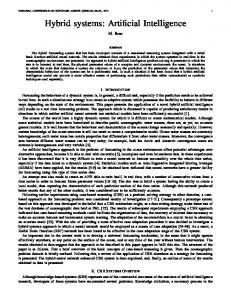
where 𝑁𝑖 is the current population size, 𝑇 𝐵𝑟𝑎𝑛𝑐ℎ is the branching threshold, 𝑤𝑖 is the branching number defined by (5), and T Nmority is the death threshold. 2.2. Root-to-Root Communication. The intrinsic property of the “population” in swarm intelligence is collective intelligence emerging by a number of connected individuals exchanging information in some specific topologies [27–30]. This means that the spatial topological structure plays an important role in enhancing dynamic interaction between individuals and optimizing information propagation path across the structured population. Accordingly, the population topology technique has been strongly recommended for potential improvement of swarm intelligence or evolutionary algorithms [30–33]. Particularly, by lucubrating on the relationship between population topologies structure and algorithmic performances in [29], Kennedy and Mendes conclude that the Von Neumann exhibits better convergence speed on a variety of test functions, as shown Figures 1(a) and 1(b). In ARFO, (3) shows that an individual’s candidate neighborhood termed 𝑥𝑙𝑏𝑒𝑠𝑡 is selected from the entire population, which indicates one central node influences, and is influenced by all other members of the population [26]. In other words, this population topological structure of ARFO essentially falls into the star topology, which is a fully connected neighborhood relation, as shown in Figure 1(c). From [29], it is claimed that the Von Neumann has a lower connectivity while covers a

4

Computational Intelligence and Neuroscience

(a) Three-dimensional Neumann

Von

(b) Two-dimensional Von Neumann

(c) Star

Figure 1: Population topology.

Von Neumann Split population of 𝑃 roots into 𝑀 rows and 𝑁 cols, and 𝑃 = 𝑀 ∗ 𝑁. Begin For 𝑖 = 1 : 𝑁 𝑥𝑖4 (𝑖, 1) = (𝑖 − Cols) mod 𝑁; If 𝑥𝑖4 (𝑖, 1) == 0 𝑥𝑖4 (𝑖, 1) = 𝑁; 𝑥𝑖4 (𝑖, 2) = 𝑖 − 1; If (𝑖 − 1) mod Cols == 0 𝑥𝑖4 (𝑖, 2) = 𝑖 − 1 + Cols; 𝑥𝑖4 (𝑖, 3) = 𝑖 + 1; If 𝑖 mod Cols == 0 𝑥𝑖4 (𝑖, 3) = 𝑖 + 1 − Cols; 𝑥𝑖4 (𝑖, 4) = (𝑖 + Cols) mod 𝑁; If 𝑥𝑖4 (𝑖, 4) == 0 𝑥𝑖4 (𝑖, 4) = 𝑁; End Algorithm 1: The pseudocode of Von Neumann.

larger search space than the star type, which tends to maintain better diversity of population and reduces the chances of falling into local optima. The procedures of representing Von Neumann structure are listed in Algorithm 1. 2.3. Coevolution Mechanism. Hierarchy is a common phenomenon in the development of plant root system [25, 26]. With the severity of environmental stress, homogeneous main roots continuously self-grow-branch and evolve while being a part of heterogeneous roots of different plant types and that plant is in turn a part of a specific ecosystem niche [27]. As a result, this hierarchical coevolution approach is incorporated to improve algorithm efficiency via decomposing large-scale problems into simple tasks optimized in parallel. As depicted in Figure 2, the flat ARFO is structured into two levels with different topologies as follows. Hypothesize that population 𝑃 = {𝑆1 , 𝑆2 , . . . , 𝑆𝑀}, and each swarm 𝑆𝑘 = {𝑥1 , 𝑥2 , . . . , 𝑥𝑁}. In each growth phase, the new individual or agent in level 2 is defined as 𝑡−1 − 𝑥𝑖𝑡−1 ) + 𝑙2 ⋅ rand2 𝑥𝑖𝑡 = 𝑥𝑖𝑡−1 + 𝑙1 ⋅ rand1 ⋅ (𝑥𝑖𝑏𝑒𝑠𝑡 𝑡−1 ⋅ (𝑥𝑝𝑏𝑒𝑠𝑡 − 𝑥𝑖𝑡−1 ) ,

(9)

P2

Top 1

P3

Level 1 P1

Pn

Level 2

Top 1: topology in level 1 Top 1, 1,. . ., Top 1, m: topology in level 2

Top 1, m

Top 1, 1

···

Population in level 1 Roots in level 2

Figure 2: Multispecies coevolution mechanism.

𝑡−1 where 𝑥𝑖𝑏𝑒𝑠𝑡 is the best individual within current population 𝑡−1 is the global which denotes cooperation in level 2 and 𝑥𝑝𝑏𝑒𝑠𝑡 best individual among all populations which exchanges

Computational Intelligence and Neuroscience

5

Initialization Initialize 𝑀 root populations, each consists of 𝑁 individuals. And set the maximum iteration number MaxT. Set 𝑡 = 0. Calculate auxin concentration values of all populations by (2). While (terminal conditions not satisfied) Divide each population into main root and lateral root groups according to auxin concentration. For each population 𝑃𝑖 Construct Von Neumann topology as shown in Algorithm 1. For each main roots group Implement regrowing operator by (9). Evaluate auxin concentration values of renewal main roots, and apply greedy selection. If the condition of branching determined by (4) is met, continue; otherwise, go to lateral-roots loop. Calculate the branching number by (5), and branching new roots by (6). Adjust the population size. End for Loop over each mainroot tip For each Lateral-roots group. Lateral-root take regrowing operator by (7). Evaluate the auxin concentration values of the renewal lateral roots, apply greedy selection. Adjust the corresponding nutrient concentration value by (2); End for Loop over each root tip of lateral-roots Remove the dead individuals from each population according to their auxin concentration values by (8). Loop over each population 𝑡 = 𝑡 + 1; End while Output the best result.

Algorithm 2: The pseudocode of HARFO.

information across populations in level 1. 𝑙1 and 𝑙2 are the random coefficients. rand1 and rand2 are random numbers with uniform distribution in [0, 1], respectively. 2.4. The Proposed Algorithm. By hybridizing ARFO with these complex degrees of strategies, namely, root-to-root communication and coevolution mechanism, the hybrid artificial root growth optimizer (HARFO) can regulate the trajectory of each root through the specific topology. Moreover, the evolution of population is guided by historical experience in level 2 and global best information in level 1, which can imply diversity of population. The main procedures of the proposed HARFO are listed in Algorithm 2. The flowchart of HARFO is presented in Figure 3.

3. Benchmark Test 3.1. Test Functions. For the purpose of performance comparison, the HARFO, together with other state-of-the-art metaheuristic algorithms, is evaluated on a set of test functions from basic benchmarks and CEC 2005 test beds. The definition and mathematical representation of them are available in Table 1 where 𝑓1 ∼𝑓5 are basic benchmark functions and

𝑓6 ∼𝑓10 are taken from CEC 2005 test suit, which is complex rotation and shift problem based on the basic test functions. Furthermore, in order to comprehensively evaluate the performance of the proposed algorithm, a suit of scalable shifted and rotated benchmarks from CEC 2014 test bed is employed in the test [34–36]. The dimensions, initialization ranges, and global optimum of each function (𝑓11 ∼𝑓20 ) are listed in Table 2. 3.2. Experimental Configuration. For the purpose of performance comparison, the HARFO is compared with several classical evolutionary algorithms including particle swarm optimization (PSO) [37, 38], cooperative coevolution genetic algorithm (CCGA) [39], pure artificial root foraging optimization algorithm (ARFO) [22], and artificial bee colony algorithm (ABC) [20] on ten test benchmarks given above. Specifically, CCGA is a parallelized GA variant derived from the dimension-distributed coevolution mode, which divides a high-dimensional problem into several lower-dimensional subproblems and then assigns them to corresponding subswarms to coevolve [39]. On each function, the algorithm is independently run 20 times and terminated when the

6

Computational Intelligence and Neuroscience Initialize M populations (Pi , i ∈ [1 : M]), each possess N individuals (Sij, i ∈ [1 : M], j ∈ [1 : N])

Set iterations number t = 0

Level 2

S11

···

S1N

···

···

S2N

SM1

···

SMN

Construct Von Neumann topology

Construct Von Neumann topology

Main root operation: regrow and branch

Main root operation: regrow and branch

Main root operation: regrow and branch

Lateral root operation

Lateral root operation

Lateral root operation

Dead root elimination

Dead root elimination

Dead root elimination

Population 1: P1

Level 1

S21

Construct Von Neumann topology

Population 2: P2

Population M: PM

Construct star topology

Update pbest if necessary

t=t+1

Criterion satisfied?

No

Yes End

Figure 3: The flowchart of HARFO algorithm.

number of function evaluations reaches 100,000 for each run. The common population size associated with ARFO, PSO, and ABC is set to 20. For PSO, the global version with inertia weight is adopted, and its parameters directly follow the default setting of [37, 38]: the acceleration factors 𝑐1 = 𝑐2 = 2.0 and the decaying inertia weight 𝜔 starting at 0.9 and ending at 0.4. For ABC, the limit is set to 𝑆𝑁 × 𝐷, where 𝐷 is the dimension of the problem and SN is half of population size [20]. For CCGA, the subswarm number is set to 10, and other parameters are the same as its original literature [39]. The parameter setting

of HARFO and ARFO can be empirically summarized in Table 3. For the proposed HARFO, the population number 𝑁, the branching, and dead thresholds should be tuned firstly in next section. 3.3. Parameters Sensitivity (i) Sensitivity in relation to Population Number 𝑀 in Level 1. To scientifically assess the effect of parameter 𝑀, the following experiment is designed. First, 𝑇 𝐵𝑟𝑎𝑛𝑐ℎ and 𝑇 𝑁𝑚𝑜𝑟𝑖𝑡𝑦 are assigned empirically with initial values 10 and 5, respectively.

Computational Intelligence and Neuroscience

7

Table 1: Parameters of basic benchmarks and CEC 2005 benchmarks (𝑥∗ is the optimal solution, 𝑓(𝑥∗ ) is the best values of function). 𝑓

Functions

Dimensions

Initial range

𝑥*

𝑓(𝑥* )

𝑓1 𝑓2 𝑓3 𝑓4 𝑓5 𝑓6 𝑓7 𝑓8

Sphere function Rosenbrock function Rastrigrin function Schwefel function Griewank function Shifted Sphere Function Shifted Rosenbrock’s Function Shifted Schwefel’s Problem Shifted Rotated Griewank’s Function without Bounds Shifted Rastrigin’s Function

20 20 20 20 20 20 20 20

[−100, 100]𝐷 [−30, 30]𝐷 [−5.12, 5.12]𝐷 [−500, 500]𝐷 [−600, 600]𝐷 [−100, 100]𝐷 [−100, 100]𝐷 [−100, 100]𝐷

[0, 0, . . . , 0] [1, 1, . . . , 1] [0, 0, . . . , 0] [420.9867, . . . , 420.9867] [0, 0, . . . , 0] [0, 0, . . . , 0] [0, 0, . . . , 0] [0, 0, . . . , 0]

0 0 0 0 0 −450 390 −450

20

No bounds

[0, 0, . . . , 0]

−180

20

[−5, 5]𝐷

[0, 0, . . . , 0]

−330

𝑓9 𝑓10

Table 2: Parameters of CEC 2014 test functions (𝑥∗ is the optimal solution; 𝑓(𝑥∗ ) is the best values of function; and 𝑂𝑖 is the shifted global optimum defined in “shift data x.txt,” which is randomly distributed in [−80, 80]𝐷 ). 𝑓 𝑓11 𝑓12 𝑓13 𝑓14 𝑓15 𝑓16 𝑓17 𝑓18 𝑓19 𝑓20

Functions Rotated High Conditioned Elliptic Function Rotated Bent Cigar Function Rotated Discus Function Shifted and Rotated Rosenbrock’s Function Shifted and Rotated Ackley’s Function Shifted and Rotated Weierstrass Function Shifted and Rotated Griewank’s Function Shifted Rastrigin’s Function Shifted and Rotated Rastrigin’s Function Shifted Schwefel’s Function

Dimensions

Initial range

𝑥*

𝑓(𝑥* )

30

[−100, 100]𝐷

𝑂1

100

30 30

[−100, 100]𝐷 [−100, 100]𝐷

𝑂2 𝑂3

200 300

30

[−100, 100]𝐷

𝑂4

400

30

[−100, 100]𝐷

𝑂5

500

30

[−100, 100]𝐷

𝑂6

600

30

[−100, 100]𝐷

𝑂7

700

30

[−100, 100]

𝐷

𝑂8

800

30

[−100, 100]𝐷

𝑂9

900

𝐷

𝑂10

1000

30

Table 3: Parameters of HARFO and ARFO for optimization. HARFO The number of initial population The maximum number of population T Branch T Nmority 𝑆𝑚𝑎𝑥 𝑆𝑚𝑖𝑛 Population number The number of initial population The maximum number of single population BranchG Nmority 𝑆𝑚𝑎𝑥 𝑆𝑚𝑖𝑛

20 100 10 5 4 1 8 4 50 10 5 4 1

[−100, 100]

Then 𝑀 is varied from 2 to 17 with a step size 3. For each value of 𝑀, HARFO is implemented for 20 times on six selected 30-dimensional 𝑓11 , 𝑓12 , 𝑓13 , 𝑓14 , and 𝑓15 . And computation results in terms of mean and standard deviation are given in Table 4. It can be visibly observed from Table 4 that algorithm with 𝑀 equal to 2 and 8 can perform superior to that with other 𝑀 values. Compared with 𝑀 = 2, the result of algorithm with 𝑀 = 8 is relatively better on three of five test benchmarks. Therefore, the optimal setting of the parameter 𝑀 can be 𝑀 = 8 as general usage of the algorithm. (ii) Sensitivity in relation to T Branch and T Nmority in Level 2. 𝑇 𝐵𝑟𝑎𝑛𝑐ℎ and 𝑇 𝑁𝑚𝑜𝑟𝑖𝑡𝑦 play vital roles in the population varying process, and there are critical correlations between them; thus, these two parameters are analyzed together. In this experiment, population number 𝑀 is fixed to 8, and the values of 𝑇 𝐵𝑟𝑎𝑛𝑐ℎ are varied as 5, 10, and 15 while the

8

Computational Intelligence and Neuroscience Table 4: Results obtained by HARFO with different population number. 𝑀

𝑓11 𝑓12 𝑓13 𝑓14 𝑓15

Mean Std Mean Std Mean Std Mean Std Mean Std

2 1.9663E + 01 6.5353E − 01 6.5523E + 01 1.1212E + 02 3.1865E + 01 1.0089E + 01 3.7411E + 01 9.6699E − 01 7.9732E + 01 3.3109E + 01

5 3.0644E + 01 7.3232E − 01 7.3533E + 01 1.2511E + 02 3.5876E + 01 1.9254E + 01 4.1955E + 01 1.0881E + 00 8.9323E + 01 3.7102E + 01

8 2.0535E + 01 4.9023E − 01 4.9234E + 01 8.4181E + 01 3.7405E + 01 1.2886E + 01 2.8088E + 01 7.2544E − 01 5.9839E + 01 2.4897E + 01

11 3.4134E + 01 8.1423E − 01 8.1788E + 01 1.3922E + 02 6.2144E + 01 2.1429E + 01 4.6603E + 01 1.2127E + 00 9.9226E + 01 4.1900E + 01

14 3.7901E + 01 9.0482E − 01 9.0872E + 01 1.5537E + 02 6.9037E + 01 2.3784E + 01 5.1842E + 01 1.3389E + 00 1.1045E + 02 4.5952E + 01

17 3.4393E + 01 8.2108E − 01 8.2462E + 01 1.4099E + 02 6.2648E + 01 2.1583E + 01 4.7044E + 01 1.2150E + 00 1.0022E + 02 4.1699E + 01

Table 5: Results obtained by HARFO with different T Branch and T Nmority. T Branch/T Nmority Mean 𝑓11 Std Mean 𝑓12 Std Mean 𝑓13 Std Mean 𝑓14 Std Mean 𝑓15 Std

5/0 2.9494E + 01 6.0931E − 01 4.5534E + 02 2.3424E + 02 3.0352E + 01 4.0945E + 01 4.0333E + 01 7.9834 1.0934E + 02 4.2213E + 02

10/0 2.9835E − 01 3.9945 2.4346E + 03 1.5529E + 02 6.3321E + 01 8.0345E + 01 1.4452E + 02 6.8554 5.5423E + 01 4.7775E + 01

relevant 𝑇 𝑁𝑚𝑜𝑟𝑖𝑡𝑦 is selected to be 0 or 5. From Table 5, it is clearly visible that the HARFO obtains best computation results on most test functions including 𝑓11 , 𝑓13 , 𝑓14 , and 𝑓15 when 𝑇 𝐵𝑟𝑎𝑛𝑐ℎ/𝑇 𝑁𝑚𝑜𝑟𝑖𝑡𝑦 are set as 10/5. Therefore, the optimal configuration of 𝑇 𝐵𝑟𝑎𝑛𝑐ℎ/𝑇 𝑁𝑚𝑜𝑟𝑖𝑡𝑦 is 10/5 as general usage of the algorithm. As the summary of this section, all suggested values of the control parameters can be listed as follows: 𝑀 = 8, 𝑇 𝐵𝑟𝑎𝑛𝑐ℎ = 10, and 𝑇 𝑁𝑚𝑜𝑟𝑖𝑡𝑦 = 5. These values are determined by experiments where the correlative 𝑇 𝐵𝑟𝑎𝑛𝑐ℎ and 𝑇 𝑁𝑚𝑜𝑟𝑖𝑡𝑦 in level 2 are taken into consideration together, and the third one in level 1 is varied over an interval with a step size. 3.4. Computational Results (i) Comparative Results on 30-Dimensional Case. HARFO is compared with ABC, PSO, and CCGA on ten 30-dimensional benchmarks 𝑓1 –𝑓10 . On each benchmark, these algorithms are independently implemented 20 times and terminated when the number of function evaluations reaches 100,000 for each run. The statistical results in terms of mean and standard deviation of each benchmark over 20 runs are calculated and shown in Table 6. As revealed from experimental results in Table 6, HARFO generally shows relative outperformance for solving most test benchmarks, compared to CCGA and

15/0 1.7934E + 01 6.1453E − 01 8.6729E − 01 3.4031E + 01 3.6239E + 01 2.9023E + 01 4.8845E + 02 5.2231E + 01 4.9000E + 01 6.0003E + 01

5/5 2.0332E + 01 5.0094E − 01 2.4621E + 02 1.6436E + 02 3.1234E + 02 9.0945E + 01 2.0340E + 02 2.4442E + 01 2.2454E + 02 8.8896E + 01

10/5 1.6815E + 01 4.0143E − 01 4.0316E + 01 6.8932E + 01 3.0629E + 01 1.0552E + 01 2.3000E + 01 5.9403E − 01 4.9000E + 01 2.0387E + 01

15/5 3.0914E + 02 9.0093 3.4344E + 01 5.6987 1.0342E + 02 9.0934E + 01 2.4136E + 00 5.9453E − 01 1.0043E + 02 3.2009E + 01

ABC, which obtain the second and third best rankings, respectively. On 𝑓1 , HARFO, CCGA, and ABC perform close to each other, relatively better than other algorithms. Specifically, CCGA does better than ABC, followed by CCGA. On 𝑓2 , ARFO remarkably outperforms others as well as CCGA and ABC obtain close results, significantly better than other algorithms. For complex multimodal variable-separable 𝑓3 , variable-separable 𝑓4 , and nonseparable 𝑓5 , HARFO performs slightly better than CCGA and ABC, furthermore significantly better than other algorithms. Particularly, on 𝑓3 and 𝑓5 , the search performance order can be shown apparently as HARFO > CCGA > ABC > ARFO > PSO. On 𝑓6 –𝑓10 , which are more complex shifted and rotated benchmarks, HARFO can obtain best performance in terms of mean, maximum, and minimum on most of five benchmarks including 𝑓6 , 𝑓8 , 𝑓9 , and 𝑓10 and ARFO also outperforms other algorithms on 𝑓7 . Apparently, HARFO shows significant improvement over other algorithms, especially ARFO. (ii) Comparative Results on 100-Dimensional Case. In order to assess the scalability of our proposed algorithm, which is crucial for its applicability to real-world high-dimensional problems, the test benchmarks are extended to 100-dimensional problems as high-dimensional cases. The experimental results are given in Table 7. From Table 7, it is observed that

Computational Intelligence and Neuroscience

9

Table 6: Comparison of results with 30 dimensions obtained by each algorithm (𝑓(𝑥) − 𝑓(𝑥∗ )). Func. Mean Std Mean Std Mean Std Mean Std Mean Std Mean Std Mean Std Mean Std Mean Std Mean Std

𝑓1 𝑓2 𝑓3 𝑓4 𝑓5 𝑓6 𝑓7 𝑓8 𝑓9 𝑓10

HARFO 4.2817E − 13 5.8831E − 13 7.2733E − 01 1.5903E + 00 2.1575E − 13 1.2233E − 12 7.6514E − 04 6.3836E − 04 5.0157E − 03 4.9156E − 03 4.0543E − 14 3.4998E − 14 8.4784E + 00 1.2762E + 00 1.9573E + 02 4.6811E + 02 1.6015E + 03 6.9952E − 01 6.8062E + 00 6.4614E − 01

ABC 1.3230E − 20 4.3300E − 20 3.9681E + 00 3.7709E + 00 4.9539E + 01 1.3063E + 01 2.8590E − 04 2.7604E − 04 8.3921E − 02 7.3446E − 02 7.5624E − 14 3.0806E − 14 2.4324E + 01 7.1995E + 01 9.0699E + 02 5.8412E + 02 2.0949E + 03 7.4802E − 13 5.9028E + 01 1.7745E − 01

ARFO 8.4537E − 03 6.6176E − 03 6.9380E + 01 1.3271E + 00 7.5788E + 01 1.1519E + 00 4.4610E + 03 2.2428E + 02 9.2917E − 01 2.8713E − 01 6.3095E + 02 7.8376E + 02 1.4680E + 00 2.0352E + 00 1.9471E + 02 1.5947E + 01 5.2497E + 03 5.2374E + 02 3.4875E + 02 6.5806E + 01

PSO 6.4050E − 01 2.2735E − 01 2.6402E + 02 1.4057E + 02 1.3201E + 02 3.7770E + 02 2.9702E + 02 2.1757E + 02 3.9481E + 00 2.6640E − 03 9.4363E + 01 3.9237E + 01 7.0365E + 06 2.3168E + 07 2.0902E + 04 4.8404E + 03 2.5180E + 03 3.8381E + 02 6.6128E + 01 5.7449E + 00

CCGA 1.2942E − 20 4.2357E − 20 3.8817E + 00 3.6888 4.8976E + 01 1.2903E + 01 2.8094E − 04 1.5404E − 04 8.2891E − 02 7.2544E − 02 7.4696E − 14 6.6428E − 14 2.4025E + 01 7.1111E + 01 8.9575E + 02 5.7698E + 02 2.0664E + 03 7.6612E − 13 5.8311E + 01 1.7554E − 01

Table 7: Comparison of results with 100 dimensions obtained by each algorithm (𝑓(𝑥) − 𝑓(𝑥∗ )). Func. 𝑓1 𝑓2 𝑓3 𝑓4 𝑓5 𝑓6 𝑓7 𝑓8 𝑓9 𝑓10

Mean Std Mean Std Mean Std Mean Std Mean Std Mean Std Mean Std Mean Std Mean Std Mean Std

HARFO 1.2867E − 03 6.2167E − 03 2.3158E + 02 2.9080E + 01 6.7884E + 02 1.3927E + 02 1.7000E + 01 4.0850E + 00 1.7451E − 01 2.1547E − 01 6.4416E + 03 1.1540E + 03 3.3781E + 10 1.1606E + 10 1.2057E + 05 1.7588E + 04 1.5149E + 03 1.0312E + 02 2.2175E + 02 3.7382E + 00

ABC 2.5048E − 03 5.0736E − 03 6.2667E + 02 6.8733E + 02 1.4622E + 02 1.8944E + 01 5.1011E + 02 1.2089E + 02 5.4011E + 01 2.7978E + 01 7.2900E + 04 2.5311E + 03 2.8028E + 10 8.0320E + 09 3.5396E + 05 9.1560E + 04 1.8168E + 04 2.7420E + 03 6.5384E + 03 3.6678E + 00

HARFO significantly outperforms other algorithms almost all test functions except for 𝑓2 and 𝑓7 . Particularly, compared to other algorithms, the solution accuracy of HARFO on shifted and rotated 𝑓5 , 𝑓9 , and 𝑓10 is increased by one order of magnitude. From the distinct difference between dimension = 20 and 100 results, it is clearly observed that with

ARFO 4.3104E − 02 7.8429E − 03 6.0868E + 02 3.3206E + 01 9.1064E + 02 6.6473E + 01 1.7000E + 01 2.3858E + 00 1.6357E + 01 4.4982E + 00 9.8642E + 03 1.0969E + 03 1.1095E + 09 4.6126E + 08 1.2118E + 05 4.1061E + 03 3.5279E + 04 1.3535E + 03 1.1434E + 03 1.2423E + 02

PSO 4.5449E + 02 1.1368E + 02 1.0874E + 04 6.7649E + 04 5.6672E + 03 7.2860E + 02 1.7000E + 01 7.2467E + 00 1.5808E + 03 3.2400E + 02 2.3474E + 05 4.0396E + 04 6.8711E + 09 1.9879E + 08 4.5362E + 05 3.1074E + 04 2.8477E + 04 8.9127E + 02 1.8442E + 03 2.2994E + 02

CCGA 1.2558E − 02 5.7436E − 03 9.8880E + 01 3.2121E + 01 8.8089E + 02 6.7302E + 01 1.8874E + 01 2.6488E + 00 1.7160E − 01 1.9940E − 01 9.5026E + 03 1.1567E + 03 1.1688E + 09 4.4435E + 08 1.3464E + 05 4.5623E + 03 3.9199E + 04 1.5039E + 03 1.2704E + 03 1.3803E + 02

dimensionality increasing, the proposed algorithm exhibits its persistence and performs better. Finally, the performance improvement obtained by our proposed algorithm can be generally explained: when other algorithms are trapped in the local optima, the HARFO can utilize the root-to-root communication mechanism

10

Computational Intelligence and Neuroscience Table 8: Comparison of results with 30 dimensions obtained by each algorithm (𝑓(𝑥) − 𝑓(𝑥∗ )). Func.

𝑓11 𝑓12 𝑓13 𝑓14 𝑓15 𝑓16 𝑓17 𝑓18 𝑓19 𝑓20

Mean Std Mean Std Mean Std Mean Std Mean Std Mean Std Mean Std Mean Std Mean Std Mean Std

HARFO 1.6815E + 01 3.9994E − 01 3.1528E + 01 2.4023E + 01 2.8969E + 01 1.5290E + 00 2.2457E + 01 4.8265E − 01 4.2697E + 01 8.1373E + 00 3.1060E − 03 1.5530E − 03 6.1585E − 06 3.3153E − 05 2.1913E + 03 4.7034E + 02 4.7272E + 02 2.2216E + 02 2.4618E + 02 1.2685E + 01

ABC 1.9799E + 07 6.7129E + 06 7.5904E + 02 7.5572E + 02 1.3000E + 01 2.5348E + 01 2.4494E + 01 4.8600E − 02 1.9000E + 01 1.7665E + 00 1.3200E − 03 3.8400E − 03 5.1208E + 02 1.1126E + 02 6.1602E + 06 3.4051E + 06 1.6622E + 04 1.4328E + 03 2.7362E + 02 1.6578E + 02

to escape. By employing the hierarchical multipopulation coevolution, the complex task is decomposed into smallerscale subproblems. (iii) Comparative Results on 30-Dimensional CEC 2014 Case. Computation results in terms of means and stand deviations of the 20 runs obtained by six algorithms on ten 30dimensional CEC 2014 benchmarks are given in Table 8, within which the best results among those algorithms are highlighted. From Table 8, the proposed HARFO performs significantly superior to its counterparts including CCGA and ABC on most of test benchmarks. Specifically, HARFO can do better than CCGA on 𝑓11 , 𝑓12 , 𝑓14 , 𝑓16 , 𝑓17 , 𝑓19 , and 𝑓20 , followed by ABC and ARFO, PSO cannot obtain competitive results. On 𝑓13 and 𝑓15 , ABC and CCGA perform significantly better than ARFO and slightly better than HARFO. PSO also obtains best result on 𝑓18 . Furthermore, we can observe that although the shifted and rotated CEC 2014 benchmarks become more difficult to be handled compared with their classical counterparts and the computation results are not as satisfactory as those in the classical benchmarks, HARFO still performs more powerful than other algorithms on most test cases. This essentially indicates that HARFO has greater potential to cope with more complex problems.

4. Real-World Application for Image Segmentation 4.1. Otsu Criterion. The well-known Otsu criterion has been widely adopted to determine the optimal thresholds with

ARFO 1.2573E + 07 1.0473E + 07 1.0104E + 08 2.3503E + 08 1.5265E + 02 5.0791E + 01 2.4296E + 01 1.2623E − 02 3.6291E + 01 3.1039E + 00 5.6546E + 00 7.0040E + 00 1.5884E + 02 3.0743E + 01 3.5613E + 05 7.1417E + 05 8.5742E + 02 1.2094E + 02 2.9471E + 02 9.1791E + 02

PSO 2.9358E + 08 2.1609E + 08 7.0153E + 08 2.8266E + 08 4.5742E + 02 1.5825E + 02 2.5464E + 01 7.6957E − 02 5.0531E + 01 2.2499E + 00 1.2402E + 02 3.0668E + 01 3.1284E + 02 4.1798E + 01 2.0148E + 03 3.4323E + 02 7.3078E + 06 5.5582E + 06 4.7931E + 02 2.9374E + 01

CCGA 1.9563E + 02 6.6330E + 02 7.5001E + 02 7.4673E + 02 1.3000E + 01 2.8136E + 01 2.7188E + 01 5.3946E − 02 1.9000E + 01 1.0608E + 00 1.4652E − 03 4.4330E − 03 5.9117E + 02 1.2844E + 02 7.1116E + 06 3.9310E + 06 1.5327E + 04 1.3212E + 03 2.5231E + 02 1.5287E + 02

desired characteristics through computing between-class variance [7, 8]. The original procedures of Otsu can be listed as below: at the beginning, a given image consisting of 𝑁 pixels of gray levels falling into the range [0, 𝐿−1] is taken into consideration. ℎ(𝑖) donates the pixel number of gray-level 𝑖 and 𝑃(𝑖) represents the probability of gray-level 𝑖. Then, we have

𝐿−1

𝑁 = ∑ ℎ (𝑖) , 𝑖=0

𝑃 (𝑖) =

(10)

ℎ (𝑖) , 𝑁 for 0 ≤ 𝑖 ≤ 𝐿 − 1.

Hypothesize that 𝑀 − 1 thresholds, namely, {𝑡1 , 𝑡2 , . . . , 𝑡𝑀−1 }, are required to segment the given image into 𝑀 classes: 𝐶1 for [0, . . . , 1], 𝐶2 for [𝑡1 +1, . . . , 1], . . ., 𝐶𝑀 for [𝑡𝑀−1 , . . . , 𝐿], ∗ the optimal thresholds {𝑡1∗ , 𝑡2∗ , . . . , 𝑡𝑀−1 } selected by Otsu are described as ∗ {𝑡1∗ , 𝑡2∗ , . . . , 𝑡𝑀−1 } = arg max {𝜎𝐵2 (𝑡1 , 𝑡2 , . . . , 𝑡𝑀−1 )} ,

0 ≤ 𝑡1 ≤ 𝑡2 ≤ ⋅ ⋅ ⋅ ≤ 𝑡𝑀−1 ≤ 𝐿,

(11)

Computational Intelligence and Neuroscience

11

Table 9: Objective values and thresholds by the Otsu method. 𝑀−1=2 Objective values Optimal thresholds Avion 3.493𝐸 + 3 113, 173 House 2.24𝐸 + 3 107, 173 Lena 9.34𝐸 + 3 134, 165, Peppers 9.35𝐸 + 3 134, 176 Safari04 2.53𝐸 + 3 82, 141 Hunter 5.45𝐸 + 3 102, 146 Mean CPU time 2.1472 Image

𝑀−1=3 Objective values Optimal thresholds 3.13𝐸 + 4 93, 145, 191 2.42𝐸 + 4 84, 137, 181 1.13𝐸 + 4 121, 151, 176 1.13𝐸 + 4 113, 158, 184 2.33𝐸 + 4 65, 107, 151 5.45𝐸 + 3 86, 129, 155 175.776

where 2

𝑀

𝜎𝐵2 = ∑𝑤𝑖 ∗ (𝑢𝑖 − 𝑢𝑡𝑖∗ ) , 𝑖=1

𝑤𝑖 = ∑ 𝑘 ∗ 𝑃𝑘 , 𝑘∈𝐶𝑖 𝐿=1

𝑢𝑖 = ∑ 𝑘 ∗ 𝑘∈𝐶𝑖

(12) 𝑃𝑘 , 𝑤𝑖 𝑖 = 1, 2, . . . , 𝑀.

Generally, (11) is employed as the fitness function for heuristic methods based procedure to be optimized. A close look into this equation will show that it is very similar to the expression for uniformity measure [40–43]. 4.2. Experiment Setup. The image segmentation experiments by HARFO are conducted on a set of image datasets. These datasets consist of a variety of standard tested images widely employed in previous studies [42–47], including avion.ppm, house.ppm, lena.ppm, peppers.ppm, safari04.ppm, and hunter.pgm with pixels size of 512 ∗ 512 (available at http://decsai.ugr.es/cvg/dbimagenes/). Several state-of-the-art EA algorithms are selected for comprehensive comparison, namely, HARFO, ABC [20], ARFO [22], CCGA [39], and IDPSO [12]. Particularly, the IDPSO is an existing enhanced PSO variant with intermediate disturbance searching strategy recently proposed in [12] for image segmentation, which has gained satisfactory image segmentation 𝑟 results. We will directly compare HARFO with existing computation results (i.e., for lena, peppers, and hunter) of IDPSO which have been reported in [12]. The parameters of HARFO, ABC, ARFO, PSO, and CCGA follow the optimal settings in Section 3.2. And the parameters of IDPSO are set the same as its original literature [12]. In this test, the proposed algorithm is to maximize the objective fitness within less computation time. The thresholds numbers 𝑀 − 1 are set to 2, 3, 4, 5, 7, and 9. And Figure 4 presents test images and their histograms. 4.3. Experimental Results and Analysis Case 1 (segmentation results with 𝑀 − 1 = 2, 3, 4). Table 9 lists the objective values and mean computational time found

𝑀−1=4 Objective values Optimal thresholds 3.45𝐸 + 4 84, 129, 172, 203 2.86𝐸 + 4 71, 118, 153, 186 1.26𝐸 + 4 111, 140, 158, 180 1.25𝐸 + 4 103, 140, 167, 189 2.43𝐸 + 4 55, 88, 120, 156 9.75𝐸 + 3 69, 112, 137, 158 7945.325

by pure Otsu, which are partly reported in [12]. In practical real-time application, we hope that algorithms can keep a suitable balance of running time and high accuracy [48]. As shown in Table 9, due to the exhaustive search feature, Otsu needs to consume too long CPU time while achieving a satisfactory optimal thresholding. It can be seen from Table 10 that the proposed HARFO provides generally close results in terms of objective values and standard deviation compared with ABC and ARFO on some test cases, such as avion and lena. On lena, IDPSO and CCGA perform similarly, still a little worse than HARFO. At the same time considering the relevant results form Table 9, the proposed HARFO algorithm consumes less CPU time than its counterparts, which means that HARFO shows better efficiency. Compared with other algorithms, the HARFO has coevolution mechanism to perform better global search in higher-dimensional space. Case 2 (segmentation results with 𝑀 − 1 = 5, 7, 9). Table 11 gives computational results with 𝑀 − 1 = 5, 7, and 9 in terms of average fitness and standard deviation of each algorithm. From Table 11, it is clearly observed that there are statistically significant differences between Cases 1 and 2 based on these segmentation algorithms, in aspects of both efficiency and stability. Due to the hybrid optimal strategies, HARFO exhibits obviously promising performance on this higher-dimensional segmentation case with 𝑀−1 = 5, 7, and 9. Among these methods except HARFO, the ABC method also possesses relative powerful exploration ability due to usage of the scout bees operation. However, as shown in Table 11, as the number of segmentation thresholds increases, the results in terms of fitness values found by HARFO are significantly better than that of other methods, including the ABC algorithm. Generally, it can be concluded that HARFO performs better than other algorithms in this higherdimensional scenario.

5. Conclusions This paper proposes and develops a novel bionic optimization algorithm inspired by plant root growth mechanism to solve multilevel threshold image segmentation, namely, hybrid artificial root foraging optimizer (HARFO). Based on original single-colony ARFO, the potential of HARFO to improve the

12

Computational Intelligence and Neuroscience

(b) House

(a) Avion 9000

8000

8000

7000

7000

6000

6000

2500 2000

5000

5000

1500

4000

4000

3000

3000 2000

2000

1000

1000

0

(c) Lena 3000

0

50

100

150 (a󳰀 )

200

250

300

0

1000 500 0 0

50

100

(d) Peppers

150 200 (b󳰀 )

250

0

300

50

100

(e) Safari04

300

250

300

12000

7000

2500

250

(f) Hunter

8000

3000

150 200 (c󳰀 )

10000

6000 2000

8000

5000 4000

1500

6000

3000

1000

4000

2000 500 0

2000

1000 0

50

100

150 (d󳰀 )

200

250

300

0

0

50

100

150 200 (e󳰀 )

250

300

Figure 4: Test images and their histograms.

0

0

50

100

150 200 (f 󳰀 )

Computational Intelligence and Neuroscience

13

Table 10: Objective values and standard deviation by heuristic methods on Otsu algorithm. Image

𝑀−1 2

Avion

3 4 2

House

3 4 2

Lena

3 4 2

Peppers

3 4 2

Safari04

3 4 2

Hunter

3 4

HARFO 4.3909E + 04 3.8166E − 01 4.4003E + 04 2.0072E − 01 4.4031E + 04 5.9884E − 01 3.6206E + 04 3.7387E − 02 3.6371E + 04 3.5218E − 02 3.6430E + 04 1.0542E + 00 2.2663E + 04 1.0934E − 02 2.4983E + 04 8.0934E − 03 2.2742E + 04 2.6544E − 01 1.0340E + 04 4.5333E − 12 1.1322E + 04 1.4422E + 00 1.9834E + 04 9.0452E − 11 2.5866E + 04 5.6183E − 01 2.5954E + 04 9.5100E − 01 2.6005E + 04 7.0754E − 01 2.2311E + 04 0 6.5233E + 03 2.4122 6.4522E + 04 1.0222

Objective values (standard deviation) ABC ARFO CCGA 3.8752E + 04 3.8870E + 04 3.902E + 04 8.7275E − 12 1.8550E − 02 8.642E − 02 3.8839E + 04 3.8948E + 04 4.034E + 04 2.1530E − 01 1.2917E − 01 4.442E − 01 3.8889E + 04 4.4001E + 04 4.441E + 04 5.3222E − 01 9.4322E − 01 1.542E − 01 3.1941E + 04 3.2069E + 04 3.423E + 04 0.0000E + 00 7.0560E − 02 2.194E − 01 3.2082E + 04 3.2209E + 04 3.441E + 04 4.2787E − 02 2.2613E − 01 5.213E − 01 3.2137E + 04 3.2332E + 04 3.424E + 04 5.4974E − 01 7.3052E − 01 2.113E + 00 1.3928E + 04 1.0034E + 04 2.132E + 03 5.0944E − 12 5.4093E − 02 2.422E − 01 2.0233E + 04 2.1033E + 04 2.142E + 04 7.42343E − 02 4.4421E − 01 2.499E − 02 2.0003E + 04 1.9999E + 04 2.042E + 04 6.42245E − 01 5.4226 5.453 1.9533E + 04 2.0344E + 04 9.924E + 03 5.34337E − 12 7.5652E − 02 5.424E − 01 1.0125E + 04 1.1333E + 04 1.153E + 04 2.5566E − 02 2.4223E − 01 5.5301 1.9593E + 04 1.9818E + 04 1.993E + 04 9.7863E − 02 1.9887 4.522E − 01 2.2766E + 04 2.2984E + 04 2.414E + 04 0.0000E + 00 4.7684E − 02 5.252E − 01 2.2865E + 04 2.3015E + 04 2.422E + 04 3.5163E − 02 2.0405E − 01 7.532E − 01 2.2903E + 04 2.3122E + 04 2.443E + 04 1.0771E + 00 1.8869E − 01 2.0934 1.0378E + 04 1.0389E + 04 5.042E + 02 0 2.0462E − 01 5.642E − 01 3.0422E + 03 6.5222E + 03 6.043E + 03 8.4544 5.4223E − 01 5.3252 1.1444E + 04 6.8632E + 03 1.214E + 04 5.7733 5.0530 3.534

global search performance and keep diversity of population relies on the combination of the root-to-root communication and multipopulation cooperative mechanism. With rootto-root communication, information exchanging between individuals can be enhanced through different efficient topologies. With coevolution mechanism, the hierarchical spatial population driven by multipopulations is constructed to ensure that diversity of population is well kept. The comparative experiments of HARFO in comparison with several classical population based algorithms are conducted on a set of 20-dimensional and 100-dimensional benchmarks. The experimental results validate the superiority of the proposed algorithm. Finally, the HARFO is

IDPSO 3.948E + 04 1.594E − 01 4.013E + 04 5.238E − 01 4.111E + 04 2.442E − 01 3.551E + 04 5.422E − 04 3.532E + 04 7.522E − 03 3.575E + 04 5.094E − 02 9.3449E3 5.46E − 12 1.1334E4 9.095E − 12 1.2558E4 4.336E − 1 9.3515E3 1.27E − 11 1.1269E4 5.46E − 12 1.2525E4 5.45E − 12 2.363E + 04 5.414E − 02 2.309E + 04 5.522E − 01 2.442E + 04 5.720E − 02 5.4491E3 0 6.4260E3 1.774E − 1 6.9721E3 1.4463

employed to handle the image segmentation problems with multilevel threshold. Computational results achieved by this method on a suit of images dataset show that the proposed algorithm has significant potential to be a novel effective and efficient image processing approach. In our future work, we will focus on perfecting this novel optimization framework from the perspective of relevance theory.

Competing Interests The authors declare that there is no conflict of interests regarding the publication of this paper.

14

Computational Intelligence and Neuroscience Table 11: Objective value and standard deviation by the compared population based methods on Otsu algorithm.

Image

𝑀−1 5

Avion

7 9 5

House

7 9 5

Lena

7 9 5

Peppers

7 9 5

Safari04

7 9 5

Hunter

7 9

HARFO 4.2940E + 04 6.6839E − 02 4.2852E + 04 3.0811E − 02 4.2857E + 04 1.3309E − 01 3.5543E + 04 5.3886E − 01 3.5558E + 04 1.0541E − 01 3.5610E + 04 1.4416E − 01 1.2141E + 04 1.1142E − 02 1.2232E + 04 1.2534E − 01 1.2154E + 04 1.7543E − 01 2.1900E + 04 5.0443E − 02 2.1717E + 04 1.3917E − 01 2.1743E + 04 2.3165E − 01 2.5363E + 04 1.1934E − 01 2.5449E + 04 1.3396E − 01 2.5472E + 04 1.0982E − 01 1.1723E + 04 9.4823E − 02 1.1774E + 04 2.0734E − 01 1.1805E + 04 1.5995E − 01

Objective values (standard deviation) ABC ARFO CCGA 4.0947E + 04 4.2721E + 04 4.266E + 04 1.5094E + 00 1.2493E + 00 3.133E − 02 4.0972E + 04 4.2735E + 04 4.266E + 04 3.8286E + 00 1.6504E + 00 4.531E − 01 4.0986E + 04 4.2639E + 04 4.275E + 04 2.6222E + 00 5.4868E − 01 2.853E − 01 3.3854E + 04 3.5364E + 04 3.443E + 04 1.8866E + 00 5.8096E − 01 2.284E − 01 3.3895E + 04 3.5360E + 04 3.512E + 04 5.4665E + 00 1.7216E + 00 5.543E − 01 3.3919E + 04 3.5263E + 04 3.521E + 04 3.8422E + 00 1.4566E + 00 2.842 1.1077E + 04 1.1890E + 04 1.340E + 04 2.3456E + 00 6.9755E − 01 2.434E − 01 1.1144E + 04 1.1942E + 04 1.135E + 04 5.0432E + 00 8.9221E − 01 2.743 1.1424E + 04 1.2012E + 04 1.133E + 04 3.8324E + 00 1.7423E + 00 3.326 2.0668E + 04 2.1587E + 04 2.202E + 04 1.7541E + 00 2.0475E + 00 2.1408E − 01 2.0710E + 04 2.1531E + 04 1.522E + 04 2.8835E + 00 2.6158E + 00 2.244 2.0725E + 04 2.1645E + 04 1.662E + 04 2.8313 2.3470 6.354 2.4130E + 04 2.5172E + 04 2.319E + 04 6.1834E + 00 1.6155E + 00 1.542E − 01 2.4154E + 04 2.5225E + 04 2.524E + 04 4.8186E + 00 1.2653E + 00 4.563E − 01 2.4165E + 04 2.5062E + 04 2.401E + 04 1.9172E + 00 5.8804E − 01 2.536 1.1205E + 04 1.1614E + 04 1.113E + 04 4.7343E + 00 1.6177E + 00 4.562E − 01 1.1242E + 04 1.1668E + 04 1.102E + 04 4.3856E + 00 1.8600E + 00 2.326 1.1260E + 04 1.1695E + 04 1.101E + 04 3.6223E + 00 4.0659E + 00 2.563

Acknowledgments This work is supported by the National Natural Science Foundation of China under Grants nos. 61503373 and 61502318 and the Natural Science Foundation of Liaoning Province under Grants nos. 2015020002 and 2015020046.

References [1] Y. K. Lim and S. U. Lee, “On the color image segmentation algorithm based on the thresholding and the fuzzy c-means techniques,” Pattern Recognition, vol. 23, no. 9, pp. 935–952, 1990.

IDPSO 4.165E + 04 4.9845E − 02 4.243E + 04 5.325E − 01 4.293E + 04 5.535E − 01 3.468E + 04 8.653E − 02 3.574E + 04 5.524E − 01 3.341E + 04 6.751E − 01 1.3399E4 2.01E − 2 1.4418E4 4.2087 1.4984E4 6.457 1.3366E4 5.019E − 1 1.4293E4 1.1924E + 1 1.4792E4 9.3027 2.516E + 04 2.526E + 00 2.413E + 04 6.224E − 01 2.446E + 04 5.514E − 01 7.350E3 5.1693 7.752E3 9.7143 7.974E3 1.620E + 1

[2] J. Kittler and J. Illingworth, “Minimum error thresholding,” Pattern Recognition, vol. 19, no. 1, pp. 41–47, 1986. [3] T. Pun, “Entropy threshold: a new approach,” Computer Graphics and Image Processing, vol. 16, no. 3, pp. 210–239, 1981. [4] N. R. Pal and S. K. Pal, “A review on image segmentation techniques,” Pattern Recognition, vol. 26, no. 9, pp. 1277–1294, 1993. [5] R. Panda, S. Agrawal, and S. Bhuyan, “Edge magnitude based multilevel thresholding using Cuckoo search technique,” Expert Systems with Applications, vol. 40, no. 18, pp. 7617–7628, 2013. [6] A. Romero and M. Cazorla, “Topological visual mapping in robotics,” Cognitive Processing, vol. 13, supplement 1, pp. S305– S308, 2012.

Computational Intelligence and Neuroscience [7] N. Otsu, “A threshold selection method from gray-level histograms,” IEEE Transactions on Systems, Man, and Cybernetics, vol. 9, no. 1, pp. 62–66, 1979. [8] J. N. Kapur, P. K. Sahoo, and A. K. C. Wong, “A new method for gray-level picture threshold using the entropy of the histogram,” Computer Vision, Graphics, and Image Processing, vol. 29, no. 3, pp. 273–285, 1985. [9] D.-M. Tsai, “A fast thresholding selection procedure for multimodal and unimodal histograms,” Pattern Recognition Letters, vol. 16, no. 6, pp. 653–666, 1995. [10] A. K. Bhandari, A. Kumar, and G. K. Singh, “Modified artificial bee colony based computationally efficient multilevel thresholding for satellite image segmentation using Kapur’s, Otsu and Tsallis functions,” Expert Systems with Applications, vol. 42, no. 3, pp. 1573–1601, 2015. [11] A. Bouaziz, A. Draa, and S. Chikhi, “Artificial bees for multilevel thresholding of iris images,” Swarm and Evolutionary Computation, vol. 21, pp. 32–40, 2015. [12] H. Gao, S. Kwong, J. Yang, and J. Cao, “Particle swarm optimization based on intermediate disturbance strategy algorithm and its application in multi-threshold image segmentation,” Information Sciences, vol. 250, pp. 82–112, 2013. [13] P. Huang, H. Cao, and S. Luo, “An artificial ant colonies approach to medical image segmentation,” Computer Methods and Programs in Biomedicine, vol. 92, no. 3, pp. 267–273, 2008. [14] H. V. H. Ayala, F. M. D. Santos, V. C. Mariani, and L. D. S. Coelho, “Image thresholding segmentation based on a novel beta differential evolution approach,” Expert Systems with Applications, vol. 42, no. 4, pp. 2136–2142, 2015. [15] M. Sezgin and B. Sankur, “Survey over image thresholding techniques and quantitative performance evaluation,” Journal of Electronic Imaging, vol. 13, no. 1, pp. 146–168, 2004. [16] A. K. Bhandari, V. K. Singh, A. Kumar, and G. K. Singh, “Cuckoo search algorithm and wind driven optimization based study of satellite image segmentation for multilevel thresholding using Kapur’s entropy,” Expert Systems with Applications, vol. 41, no. 7, pp. 3538–3560, 2014. [17] P. D. Sathya and R. Kayalvizhi, “Modified bacterial foraging algorithm based multilevel thresholding for image segmentation,” Engineering Applications of Artificial Intelligence, vol. 24, no. 4, pp. 595–615, 2011. [18] C. A. Coello Coello, G. T. Pulido, and M. S. Lechuga, “Handling multiple objectives with particle swarm optimization,” IEEE Transactions on Evolutionary Computation, vol. 8, no. 3, pp. 256–279, 2004. [19] A. Bishopp, H. Help, S. El-Showk et al., “A mutually inhibitory interaction between auxin and cytokinin specifies vascular pattern in roots,” Current Biology, vol. 21, no. 11, pp. 917–926, 2011. [20] D. Karaboga and B. Basturk, “On the performance of artificial bee colony (ABC) algorithm,” Applied Soft Computing, vol. 8, no. 1, pp. 687–697, 2008. [21] G. G. McNickle, C. C. St Clair, and J. F. Cahill Jr., “Focusing the metaphor: plant root foraging behaviour,” Trends in Ecology and Evolution, vol. 24, no. 8, pp. 419–426, 2009. [22] L. Ma, Y. Zhu, Y. Liu, L. Tian, and H. Chen, “A novel bionic algorithm inspired by plant root foraging behaviors,” Applied Soft Computing Journal, vol. 37, pp. 95–113, 2015. [23] L. Ma, K. Hu, Y. Zhu, and H. Chen, “A hybrid artificial bee colony optimizer by combining with life-cycle, Powell’s search and crossover,” Applied Mathematics and Computation, vol. 252, pp. 133–154, 2015.

15 [24] L. Ma, K. Hu, Y. Zhu, and H. Chen, “Cooperative artificial bee colony algorithm for multi-objective RFID network planning,” Journal of Network and Computer Applications, vol. 42, pp. 143– 162, 2014. [25] H. Wang, Y. Inukai, and A. Yamauchi, “Root development and nutrient uptake,” Critical Reviews in Plant Sciences, vol. 25, no. 3, pp. 279–301, 2006. [26] Z. Wang, M. van Kleunen, H. J. During, and M. J. A. Werger, “Root foraging increases performance of the clonal plant Potentilla reptans in heterogeneous nutrient environments,” PLoS ONE, vol. 8, no. 3, Article ID e58602, 2013. [27] M. Dannowski and A. Block, “Fractal geometry and root system structures of heterogeneous plant communities,” Plant and Soil, vol. 272, no. 1-2, pp. 61–76, 2005. [28] S. W. Kembel, H. De Kroon, J. F. Cahill Jr., and L. Mommer, “Improving the scale and precision of hypotheses to explain root foraging ability,” Annals of Botany, vol. 101, no. 9, pp. 1295–1301, 2008. [29] J. Kennedy and R. Mendes, “Population structure and particle swarm performance,” in Proceedings of the Congress on Evolutionary Computation (CEC ’02), pp. 1671–1676, IEEE, May 2002. [30] S. K. Gleeson and J. E. Fry, “Root proliferation and marginal patch value,” Oikos, vol. 79, no. 2, pp. 387–393, 1997. [31] C. K. Kelly, “Resource choice in Cuscuta europaea,” Proceedings of the National Academy of Sciences of the United States of America, vol. 89, no. 24, pp. 12194–12197, 1992. [32] H. de Kroon, H. Huber, J. F. Stuefer, and J. M. van Groenendael, “A modular concept of phenotypic plasticity in plants,” New Phytologist, vol. 166, no. 1, pp. 73–82, 2005. [33] J. H. Holland, Adaptation in Natural and Artificial Systems: An Introductory Analysis with Applications to B, Control, and Artificial Intelligence, University of Michigan Press, Ann Arbor, Mich, USA, 1975. [34] L. Ma, K. Hu, Y. Zhu, B. Niu, H. Chen, and M. He, “Discrete and continuous optimization based on hierarchical artificial bee colony optimizer,” Journal of Applied Mathematics, vol. 2014, Article ID 402616, 20 pages, 2014. [35] J. Liang, B. Qu, and P. Suganthan, “Problem definitions and evaluation criteria for the CEC 2014 special session and competition on single objective real-parameter numerical optimization,” Tech. Rep., Zhengzhou University, 2013. [36] J. J. Liang, A. K. Qin, P. N. Suganthan, and S. Baskar, “Comprehensive learning particle swarm optimizer for global optimization of multimodal functions,” IEEE Transactions on Evolutionary Computation, vol. 10, no. 3, pp. 281–295, 2006. [37] R. C. Eberhart and J. Kennedy, “New optimizer using particle swarm theory,” in Proceedings of the 1995 6th International Symposium on Micro Machine and Human Science, pp. 39–43, Nagoya, Japan, October 1995. [38] D. Corne, M. Dorigo, and F. Glover, New Ideas in Optimization, McGraw-Hill, New York, NY, USA, 1999. [39] M. A. Potter and K. A. De Jong, “Cooperative coevolution: an architecture for evolving coadapted subcomponents,” Evolutionary computation, vol. 8, no. 1, pp. 1–29, 2000. [40] H. Wang and Q. Ni, “A new method of moving asymptotes for large-scale unconstrained optimization,” Applied Mathematics and Computation, vol. 203, no. 1, pp. 62–71, 2008. [41] W. B. Tao, H. Jin, and L. M. Liu, “Object segmentation using ant colony optimization algorithm and fuzzy entropy,” Pattern Recognition Letters, vol. 28, no. 7, pp. 788–796, 2007.

16 [42] P.-Y. Yin, “Multilevel minimum cross entropy threshold selection based on particle swarm optimization,” Applied Mathematics and Computation, vol. 184, no. 2, pp. 503–513, 2007. [43] L. Cao, P. Bao, and Z. K. Shi, “The strongest schema learning GA and its application to multilevel thresholding,” Image and Vision Computing, vol. 26, no. 5, pp. 716–724, 2008. [44] X. Li, Z. Zhao, and H. D. Cheng, “Fuzzy entropy threshold approach to breast cancer detection,” Information Sciencesapplications, vol. 4, no. 1, pp. 49–56, 1995. [45] M.-H. Horng and R.-J. Liou, “Multilevel minimum cross entropy threshold selection based on the firefly algorithm,” Expert Systems with Applications, vol. 38, no. 12, pp. 14805–14811, 2011. [46] L. Ma and R. C. Staunton, “A modified fuzzy C-means image segmentation algorithm for use with uneven illumination patterns,” Pattern Recognition, vol. 40, no. 11, pp. 3005–3011, 2007. [47] P.-S. Liao, T.-S. Chen, and P.-C. Chung, “A fast algorithm for multilevel thresholding,” Journal of Information Science & Engineering, vol. 17, no. 5, pp. 713–727, 2001. [48] L. Ma, Y. Zhu, D. Zhang, and B. Niu, “A hybrid approach to artificial bee colony algorithm,” Neural Computing & Applications, vol. 27, no. 2, pp. 387–409, 2016.

Computational Intelligence and Neuroscience