Hybrid control of networked embedded systems A. Balluchi, L. Benvenuti, S. Engell, T. Geyer, K.H. Johansson, F. Lamnabhi-Lagarrigue∗, J. Lygeros M. Morari, G. Papafotiou, A.L. Sangiovanni-Vincentelli, F. Santucci, O. Stursberg†
Abstract Hybrid systems that involve the interaction of continuous and discrete dynamics have been an active area of research for a number of years. In this paper, we start by briefly surveying the main theoretical control problems that have been treated in the hybrid systems setting and classify them into stabilization, optimal control and language specification problems. We then provide an overview of recent developments in four of the most prominent application areas of hybrid control methods: Control of power systems, industrial process control, design of automotive electronics and communication networks.
1
Introduction
The term hybrid systems is used in the literature to refer to systems that feature an interaction between diverse types of dynamics. Most heavily studied in recent years are hybrid systems that involve the interaction between continuous and discrete dynamics. The study of this class of systems has to a large extent been motivated by applications to embedded systems and control. Embedded systems by definition involve the interaction between digital devices and a predominantly analog environment. In addition, much of the design complexity of embedded systems comes from the fact that they have to meet specifications such as hard real-time constraints, scheduling constraints, etc. that involve a mixture of discrete and continuous requirements. Therefore, both the model and the specifications of embedded systems can naturally be expressed in the context of hybrid systems. Control problems have been at the forefront of hybrid systems research from the very beginning. The reason is that many important applications with prominent hybrid dynamics come from the area of embedded control. For example, hybrid control has played an important role in applications to avionics, automated highways, communication networks, automotive control, air traffic management, industrial process control, manufacturing and robotics. In this overview paper we start by surveying and classifying the control problems that have been investigated in the hybrid systems literature (Section 2). We then discuss recent developments in four key application areas of hybrid control: control of power electronics (Section 3), industrial process control (Section 4), automotive control (Section 5) and communication systems (Section 6). We conclude the paper with a discussion of the open problems, research challenges and vistas (Section 7). ∗ Contact author, Laboratoire des Signaux et Systemes, Centre National de la Recherche Scientifique 3 rue Joliot Curie, 91192 Gif-sur-Yvette, France,
[email protected] † The work carried out in the framework of the HYCON Network of Excellence, funded by the European Commission, contract number FP6-IST-511368.
1
2
An overview of hybrid control problems
2.1
Control problem classification
The control problems that have been studied in the literature differ, first of all, in the way in which they treat uncertainty. Generally, the problems can be grouped into three classes: 1. Deterministic. Here it is assumed that there is no uncertainty; control inputs are the only class of inputs considered. 2. Non-deterministic. In this case inputs are grouped into two classes, control and disturbance. The design of a controller for regulating the control inputs assumes that disturbance inputs are adverserial. Likewise, the requirements are stated as worst case: the controller should be such that the specifications are met for all possible actions of the disturbance. From a control perspective, problems in this class are typically framed in the context of robust control, or game theory. 3. Stochastic. Again, both control and disturbance inputs are considered. The difference with the non-deterministic case is that a probability distribution is assumed for the disturbance inputs. This extra information can be exploited by the controller and also allows one to formulate finer requirements. For example, it may not be necessary to meet the specifications for all disturbances, as long as the probability of meeting them is high enough. In addition, the control problems studied in the literature differ in the specifications they try to meet: 1. Stabilization. Here the problem is to select the continuous inputs and/or the timing and destinations of discrete switches to make sure that the system remains close to an equilibrium point, limit cycle, or other invariant set. Many variants of this problem have been studied in the literature. They differ in the type of control inputs considered (discrete, continuous, or both) and the type of stability specification (stabilization, asymptotic or exponential stabilization, practical stabilization, etc.). Even more variants have been considered in the case of stochastic hybrid systems (stability in distribution, moment stability, almost sure asymptotic stability, etc.). 2. Optimal control. Here the problem is to steer the hybrid system using continuous and/or discrete controls in a way that minimizes a certain cost function. Again, different variants have been considered, depending on whether discrete and/or continuous inputs are available, whether cost is accumulated along continuous evolution and/or during discrete transitions, whether the time horizon over which the optimization is carried out is finite or infinite, etc. 3. Language specifications. Control problems of great interest can also be formulated by imposing the requirement that the trajectories of the closed-loop system are all contained in a set of desirable trajectories. Typical requirements of this type arise from reachability considerations, either of the safety type (along all trajectories the state of the system should remain in a “good” region of the state space), or of the liveness type (the state of the system should eventually reach a “good” region of the state space along all trajectories). Starting with these simple requirements, progressively more and more complex specifications can be formulated: the state should visit a given set of states infinitely often, given two sets of states, if the state visits one infinitely often it should also visit the other infinitely often, etc. These specifications are all related to the “language” generated by the closed-loop system and have been to a large extent motivated by analogous problems formulated for discrete systems based on temporal logic. In this section we present an overview of the problems that have been addressed in the literature in these classes. We start by briefly introducing some modeling concepts necessary to highlight the differences between the different problems. We then discuss stabilization, optimal control and language specification problems in separate subsections.
2
2.2
A simple hybrid control model
Hybrid control problems have been formulated for both continuous- and discrete-time systems. In this section we introduce a model suitable for formulating continuous-time control problems for hybrid systems; a class of discrete time models is introduced in Section 3. We restrict our attention to hybrid systems that do not include any probabilistic phenomena; the formal definition of stochastic hybrid models requires considerable mathematical overhead, even in the simplest cases. Since we are interested in hybrid dynamics, the dynamical systems we consider involve both a continuous state (denoted by x ∈ X = Rn ) and a discrete state (denoted by q ∈ Q). To allow us to capture the different types of uncertainties discussed above, we also assume that the evolution of the state is influenced by two different kinds of inputs: controls and disturbances. We assume that inputs of each kind can be either discrete or continuous, and we use υ ∈ Υ to denote discrete controls, u ∈ U ⊆ Rm to denote continuous controls, δ ∈ ∆ to denote discrete disturbances, and d ∈ D ⊆ Rp to denote continuous disturbances. The sets Q, Υ and ∆ are assumed to be countable or finite. The dynamics of the state are determined through four functions: a vector field f : Q × X × U × D → X that determines the continuous evolution, a reset map r : Q × Q × X × U × D → X that determines the outcome of the discrete transitions, “guard” sets G : Q × Q × Υ × ∆ → 2X that determine when discrete transitions can take place, and “domain” sets Dom : Q × Υ × ∆ → 2X that determines when continuous evolution is possible1 . To avoid pathological situations (lack of solutions, deadlock, chattering, etc.) one needs to introduce technical assumptions on the model components. Typically, these include continuity assumptionsSon f and r, compactness assumptions on U and D, and convexity assumptions on S d∈D f (q, x, u, d), etc. As for continuous systems, these assumptions aim to ensure u∈U f (q, x, u, d) and that for all q ∈ Q, x0 ∈ X and u(·), d(·) measurable functions of time, the differential equation x(t) ˙ = f (q, x(t), u(t), d(t)) has a unique solution x(·) : R+ → X with x(0) = x0 . Additional assumptions are often imposed to prevent deadlock, a situation where it is not possible to proceed by continuous evolution, or by discrete transition. Finally, in many publications assumptions are introduced to prevent what is called the Zeno phenomenon, a situation where the solution of the system takes an infinite number of discrete transitions in a finite amount of time. The Zeno phenomenon can prove particularly problematic for hybrid control problems, since it may be exploited either by the control or by the disturbance variables. For example, a controller may appear to meet a safety specification by forcing all trajectories of the system to be Zeno. This situation is undesirable in practice, since the specifications are met not because of successful controller design but because of modeling over-abstraction. The solutions of this class of hybrid systems can be defined using the notion of a hybrid time set [39]. A hybrid time set τ = {Ii }N i=0 is a finite or infinite sequence of intervals of the real line, such that for ′ ′ all i < N , Ii = [τi , τi′ ] with τi ≤ τi′ = τi+1 and, if N < ∞, then either IN = [τN , τN ], or IN = [τN , τN ), ′ possibly with τN = ∞. Since the dynamical systems considered here are time invariant, without loss of generality we can assume that τ0 = 0. Roughly speaking, solutions of the hybrid systems considered here (often called “runs”, or “executions”) are defined together with their hybrid time sets and involve a sequence of intervals of continuous evolution followed by discrete transitions. Starting at some initial state (q0 , x0 ), the continuous state moves along the solution of the differential equation x˙ = f (q0 , x, u, d) as long as it does not leave the set Dom(q0 , υ, δ). The discrete state remains constant throughout this time. If at some point x reaches a set G(q0 , q ′ , υ, δ) for some q ′ ∈ Q, a discrete transition can take place. The first interval of τ ends and the second one begins with a new state (q ′ , x′ ) where x′ is determined by the reset map r. The process is then repeated. Notice that considerable freedom is allowed when defining the solution in this “declarative” way: in addition to the effect of the input variables, there may also be a choice between evolving continuously or taking a discrete transition (if the continuous state is in both the domain set and a guard set) or between multiple discrete transitions (if the continuous state is in many guard sets at the same time). A bit more formally, a run of a the hybrid system can be defined as a collection (τ, q, x, υ, u, δ, d) consisting N of a hybrid time set τ = {Ii }N i=0 and sequences of functions q = {qi (·) : Ii → Q}i=0 , x = {xi (·) : Ii → 1 As
usual, 2X stands for the set of all subsets of X
3
X}N i=0 , etc. that satisfy the following conditions: • Discrete evolution: for i < N , 1. xi (τi′ ) ∈ G(qi (τi′ ), qi+1 (τi+1 ), υi (τi′ ), δi (τi′ )). 2. xi+1 (τi+1 ) = r(qi (τi′ ), qi+1 (τi+1 ), xi (τi′ ), ui (τi′ ), di (τi′ )). • Continuous evolution: for all i with τi < τi′ 1. ui (·) and di (·) are measurable functions. 2. qi (t) = qi (τi ) for all t ∈ Ii . 3. xi (·) is a solution to x˙ i (t) = f (qi (t), xi (t), ui (t), di (t)) over the interval Ii starting at xi (τi ). 4. xi (t) ∈ Dom(qi (t), υi (t), δi (t)) for all t ∈ [τi , τi′ ). This model allows control and disturbance inputs to influence the evolution of the system in a number of ways. In particular, control and disturbance can 1. Steer the continuous evolution through the effect of u and d on the vector field f . 2. Force discrete transitions to take place through the effect of υ and δ on the domain Dom. 3. Affect the discrete state reached after a discrete transition through the effect of υ and δ on the guards G. 4. Affect the continuous state reached after a discrete transition through the effect of u and d on the reset function r. An issue that arises is the type of controllers one allows for selecting the control inputs u and υ. The most common control strategies considered in the hybrid systems literature are, of course, static feedback strategies. In this case the controller can be thought of as a map (in general set valued) of the form g : Q × X → 2Υ×U . For controllers of this type, the runs of the closed-loop system can easily be defined as runs, (τ, q, x, υ, u, δ, d), of the uncontrolled system such that for all Ii ∈ τ and all t ∈ Ii , (υi (t), ui (t)) ∈ g(qi (t), xi (t)). It turns out that for certain kinds of control problems one can restrict attention to feedback controllers without loss of generality. For other problems, however, one may be forced to consider more general classes of controllers: dynamic feedback controllers that incorporate observers for output feedback problems, controllers that involve non-anticipative strategies for gaming problems, piecewise constant controllers to prevent chattering, etc. Even for these types of controllers, it is usually intuitively clear what one means by the runs of the closed-loop system. However, unlike feedback controllers, a formal definition would require one to formulate the problem in a compositional hybrid systems framework and formally define the closed-loop system as the composition of a plant and a controller automaton.
2.3
Stabilization of hybrid systems
For stabilization, the aim is to design controllers such that the runs of the closed-loop system remain close and possibly converge to a given invariant set. An invariant set is a set of states with the property that runs starting in the set remain in the set forever. More formally, W ⊆ Q × X is an invariant set if for all (ˆ q, x ˆ) ∈ W and all runs (τ, q, x, υ, u, δ, d) starting at (ˆ q, x ˆ), (qi (t), xi (t)) ∈ W, ∀Ii ∈ τ, ∀t ∈ Ii . The most common invariant sets are those associated with equilibria, points x ˆ ∈ X that are preserved under both discrete and continuous evolution.
4
The definitions of stability can naturally be extended to hybrid systems by defining a metric on the hybrid state space. An easy way to do this is to consider the Euclidean metric on the continuous space and the discrete metric on the discrete space (dD (q, q ′ ) = 0 if q = q ′ and dD (q, q ′ ) = 1 if q 6= q ′ ) and define the hybrid metric by dH ((q, x), (q ′ , x′ )) = dD (q, q ′ ) + kx − x′ k. The metric notation can be extended to sets in the usual way. Equipped with this metric, the standard stability definitions (Lyapunov stability, asymptotic stability, exponential stability, practical stability, etc.) naturally extend from the continuous to the hybrid domain. For example, an invariant set, W , is called stable if for all ǫ > 0 there exists ǫ′ > 0 such that for all (q, x) ∈ Q × X with dH ((q, x), W ) < ǫ′ and all runs (τ, q, x, υ, u, δ, d) starting at (q, x), dH ((qi (t), xi (t)), W ) < ǫ, ∀Ii ∈ τ, ∀t ∈ Ii . Stability of hybrid systems has been extensively studied in recent years (see the overview papers [18, 36]). By comparison, the work on stabilization problems is relatively sparse. A family of stabilization schemes assumes that the continuous dynamics are given, for example, stabilizing controllers have been designed for each f (q, ·, ·, ·). Procedures are then defined for determining the switching times (or at least constraints on the switching times) to ensure that the closed-loop system is stable, asymptotically stable, or practically stable [33, 53, 61, 64]. Stronger results are possible for special classes of systems, such as planar systems [63]. For non-deterministic systems, in [22] an approach to the practical exponential stabilization of a class of hybrid systems with disturbances is presented. For a brief overview of stabilization problems for classes of stochastic hybrid systems the reader is referred to [65].
2.4
Optimal control of hybrid systems
In optimal control problems it is typically assumed that a cost is assigned to the different runs of the hybrid system. The objective of the controller is then to minimize this cost by selecting the values of the control variables appropriately. Typically, the cost function assigns a cost to both continuous evolution and discrete transitions. For example, for the cost assigned to a run (τ, q, x, υ, u, δ, d) with τ = {Ii }N i=0 , the cost function may have the form # "Z ′ N τi X ′ l(qi (t), xi (t), ui (t), di (t))dt + g(qi (τi′ ), xi (τi′ ), qi+1 (τi+1 ), xi+1 (τi+1 ), ui (τi ), di (τi ), υi (τi′ ), δi (τi′ )) , i=0
τi
where l : Q × X × U × D → R is a function assigning a cost to the pieces of continuous evolution and g : Q × X × Q × X × U × D × Υ × ∆ → R is a function assigning a cost to discrete transitions. Different variants of optimal control problems can be formulated, depending on, e.g., the type of cost function, the horizon over which the optimization takes place (finite or infinite), or whether the initial and/or final states are specified. As with continuous systems, two different approaches have been developed for addressing such optimal control problems. One is based on the maximum principle and the other on dynamic programming. Extensions of the maximum principle to hybrid systems have been proposed by numerous authors; see [28, 54, 56]. The solution of the optimal control problem with the dynamic programming approach typically requires the computation of a value function, which is characterized as a viscosity solution to a set of variational or quasi-variational inequalities [10, 14]. Computational methods for solving the resulting variational and quasi-variational inequalities are presented in [42]. For simple classes of systems (e.g., timed automata) and simple cost functions (e.g., minimum time problems) it is often possible to exactly compute the optimal cost and optimal control strategy, without resorting to numerical approximations (see [11] and the references therein). A somewhat different optimal control problem arises when one tries to control hybrid systems using model predictive or receding horizon techniques. This approach is discussed in greater detail in Section 3, in the context of power system control. 5
2.5
Language specification problems
Another type of control problem that has attracted considerable attention in the hybrid systems literature revolves around language specifications. One example of language specifications is the safety specifications. In this case a “good” set of states W ⊆ Q × X is given and the designer is asked to produce a controller that ensures that the state always stays in this set; in other words, for all runs (τ, q, x, υ, u, δ, d) of the closed-loop system ∀Ii ∈ τ ∀t ∈ Ii , (qi (t), xi (t)) ∈ W. The name “safety specifications” (which has a formal meaning in computer science) intuitively refers to the fact that such specifications can be used to encode safety requirements in a system, to ensure that nothing bad happens, e.g., ensure that vehicles in an automated highway system (see the discussion in Section 6) do not collide with one another. Safety specifications are usually easy to meet, e.g., if no vehicles are allowed on the highway collisions are impossible. To make sure that in addition to being safe the system actually does something useful, liveness specifications are usually also imposed. The simplest type of liveness specification deals with reachability: given a set of states W ⊆ Q × X, design a controller such that for all runs (τ, q, x, υ, u, δ, d) of the closed-loop system ∃Ii ∈ τ ∃t ∈ Ii , (qi (t), xi (t)) ∈ W. In the automated highways context a minimal liveness type requirement is to make sure that the vehicles eventually arrive at their destination. Mixing different types of specifications like the ones given above one can construct arbitrarily complex properties, e.g., ensure that the state visits a set infinitely often, ensure that it reaches a set and stays there forever after, etc. Such complex language specifications are usually encoded formally using temporal logic notation. Controller design problems under language specifications have been studied very extensively for discrete systems in the computer science literature. The approach was then extended to classes of hybrid systems such as timed automata (systems with continuous dynamics of the form x˙ = 1, [4]) and rectangular automata (systems with continuous dynamics of the form x˙ ∈ [l, u] for fixed parameters l, u, [62]). For systems of this type, exact and automatic computation of the controllers may be possible using model checking tools [9, 16, 31]. In all these cases the controller affects only the discrete aspects of the system evolution, i.e., the destination and timing of discrete transitions. More general language problems (e.g., where the dynamics are linear, the controller affects the continuous motion of the system) can often be solved automatically for discrete time systems using methods from mathematical programming (see Section 3 for a discussion). Extensions to general classes of hybrid systems in continuous time have been concerned primarily with computable numerical approximations of reachable sets using polyhedral approximations [3, 15, 51], ellipsoidal approximations [13], or more general classes of sets. A useful link in this direction has been the relation between reachability problems and optimal control problems with an l∞ penalty function [58]. This link has allowed the development of numerical tools that use partial differential equation solvers to approximate the value function of the optimal control problems and hence indirectly characterize reachable sets [42].
3 3.1
Model predictive control in power electronics Control problems in power electronics
Power electronics systems represent a well-established technology that has seen significant performance improvements over the last two decades. In general, these systems are used to transform electrical power from one – usually unregulated – form to another regulated one (e.g. consider the problem of unregulated dc to regulated dc conversion). This transformation is achieved by the use of semiconductor devices that operate as power switches, turning on and off with a high switching frequency. From the control point 6
of view, power electronic circuits and systems constitute excellent examples of hybrid systems, since the discrete switch positions are associated with different continuous-time dynamics. Moreover, both physical and safety constraints are present. Power electronics circuits and systems have traditionally been controlled in industry using linear controllers combined with non-linear procedures like Pulse Width Modulation (PWM). The models used for controller design are a result of simplifications that include averaging the behavior of the system over time (to avoid modelling the switching) and linearizing around a specific operating point disregarding all constraints. As a result, the derived controller usually performs well only in a neighborhood around the operating point. To make the system operate in a reliable way for the whole operating range, the control circuit is subsequently augmented by a number of heuristic patches. The result of this procedure are large development times and the lack of theoretically backed guarantees for the operation of the system; in particular, no global stability guarantees can be given. Recent theoretical advances in the field of hybrid systems, together with the availability of significant computational power for the control loops of power electronics systems, are inviting both the control and the power electronics communities to revisit the control issues associated with power electronics applications. Such an effort for a novel approach to controlling power electronics systems is outlined in this section, where we demonstrate the application of hybrid optimal control methodologies to power electronics systems. More specifically, we show how Model Predictive Control (MPC) [40] can be applied to problems of induction motor drives and dc-dc conversion illustrating the procedure using two examples: the Direct Torque Control (DTC) of three-phase induction motors and the optimal control of fixedfrequency switch-mode dc-dc converters. The use of optimal control methodologies implies the solution of an underlying optimization problem. Given the high switching frequency that is used in power electronics applications and the large solution times that are usually needed for such optimization problems, solving this problem on-line may very well be infeasible. Depending on the application, this obstacle can be overcome in two ways; either by presolving off-line the optimization problem for the whole state-space using multi-parametric programming, a procedure that results in a polyhedral PieceWise Affine (PWA) controller that can be stored in a look-up table, or by developing solution algorithms that are dedicated, tailored to the problem and can thus be executed within the limited time available. The first approach has been followed here for the optimal control of fixed-frequency dc-dc converters, whereas the second one has been applied to the DTC problem.
3.2
Optimal control of discrete time hybrid systems
In the following, we restrict ourselves to the discrete-time domain, and we confine our models to (piecewise) affine dynamics rather than allowing general nonlinear dynamics. This not only avoids a number of mathematical problems (like Zeno behavior), but allows us to derive models for which we can pose analysis and optimal control problems that are computationally tractable. To model such discrete-time linear hybrid systems, we adopt Mixed Logical Dynamical (MLD) [8] models and the PieceWise Affine (PWA) [55] framework. Other representations of such systems include Linear Complementarity (LC) systems, Extended Linear Complementarity (ELC) systems and Max-Min-Plus-Scaling (MMPS) systems that are, as shown in [30], equivalent to the MLD and PWA forms under mild conditions. Model Predictive Control (MPC) [40] has been used successfully for a long time in the process industry and recently also for hybrid systems, for which, as shown in [8], MPC has proven to be particularly well suited. The control action is obtained by minimizing an objective function over a finite or infinite horizon subject to the evolution in time of the model of the controlled process and constraints on the states and manipulated variables. For linear hybrid systems, depending on the norm used in the objective function, this minimization problem amounts to solving a Mixed-Integer Linear Program (MILP) or Mixed-Integer Quadratic Program (MIQP). The major advantage of MPC is its straightforward design procedure. Given a (linear or hybrid) model of the system, one only needs to set up an objective function that incorporates the control objectives. 7
a
c
b
+ V2dc xc υn
ua = +1 ub = −1
xc
ias ibs ics
IM
uc = 0
− V2dc
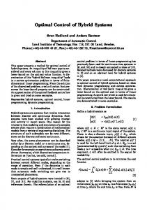
Figure 1: The equivalent representation of a three-phase three-level inverter driving an induction motor
Additional hard (physical) constraints can be easily dealt with by adding them as inequality constraints, whereas soft constraints can be accounted for in the objective function using large penalties. For details concerning the set up of the MPC formulation in connection with linear hybrid models, the reader is referred to [8] and [7]. Details about MPC can be found in [40]. To make the proposed optimal control strategies applicable to power electronics systems it is mandatory to overcome the obstacle posed by the large computation times occurring when solving the optimal control problem on-line. This can be achieved by pre-computing the optimal state-feedback control law off-line for all feasible states using the state vector as a parameter. For hybrid systems, such a method has been recently introduced, which is based on a PWA description of the controlled system and a linear objective function, using the 1- or ∞-norm. The details can be found in [6], where the authors report an algorithm that generates the solution by combining dynamic programming with multi-parametric programming and some basic polyhedral manipulations. As shown in [12], the resulting optimal state-feedback control law is a PWA function of the state defined on a polyhedral partition of the feasible state-space. More specifically, the state-space is partitioned into polyhedral sets and for each of these sets the optimal control law is given as an affine function of the state. As a result, such a state-feedback controller can be implemented easily on-line as a look-up table. Optimal direct torque control of three-phase induction motors: The rapid development of power semiconductor devices led to the increased use of adjustable speed induction motor drives in a variety of applications. In these systems, dc-ac inverters are used to drive induction motors as variable frequency three-phase voltage or current sources. One methodology for controlling the torque and speed of induction motor drives is Direct Torque Control (DTC) [57], which features very favorable control performance and implementation properties. The basic principle of DTC is to exploit the fast dynamics of the motor’s stator flux and to directly manipulate the stator flux vector such that the desired torque is produced. This is achieved by choosing an inverter switch combination that drives the stator flux vector to the desired position by directly applying the appropriate voltages to the motor windings. This choice is made usually with a sampling time Ts = 25 µs using a pre-designed switching table that is traditionally derived in a heuristic way and, depending on the particularities of the application, addresses a number of different control objectives. These primarily concern the induction motor – more specifically, the stator flux and the electromagnetic torque need to be kept within pre-specified bounds around their references. In high power applications, where three-level inverters with Gate Turn-Off (GTO) thyristors are used, the control objectives are extended to the inverter and also include the minimization of the average switching frequency and the balancing of the inverter’s neutral point potential around zero. As mentioned in the introduction, because of the discrete switch positions of the inverter, the DTC problem is a hybrid control problem, which is complicated by the nonlinear behavior of the torque, length of stator flux and the neutral point potential. We aim at deriving MPC schemes that keep the three controlled variables (torque, flux, neutral point potential) within their given bounds, minimize the (average) switching frequency, and are conceptually and computationally simple yet yield a significant performance improvement with respect to the state of the art. More specifically, the term conceptually simple refers to controllers allowing for straightforward tuning of the controller parameters or even a lack of such parameters, and easy adaptation to different
8
physical setups and drives, whereas computationally simple implies that the control scheme does not require excessive computational power to allow the implementation on DTC hardware that is currently available or at least will be so within a few years. An important first step is to derive discrete-time hybrid models of the drive tailored to our needs – or more specifically, models that are of low complexity yet of sufficient accuracy to serve as prediction models for our model-based control schemes. To achieve this, we have exploited in [48, 50] a number of physical properties of DTC drives. These properties are the (compared with the stator flux) slow rotor flux and speed dynamics, the symmetry of the voltage vectors, and the invariance of the motor outputs under flux rotation. The low-complexity models are derived by assuming constant speed within the prediction horizon, mapping the states (the fluxes) into a 60 degree sector, and aligning the rotor flux vector with the d-axis of the orthogonal dq0 reference frame rotating with the rotational speed of the rotor [35]. The benefits of doing this are a reduction of the number of states from five to three, and a highly reduced domain on which the nonlinear functions need to be approximated by PWA functions. Based on the hybrid models of the DTC drive, we have proposed in [24, 26, 50] three novel control approaches to tackle the DTC problem, which are inspired by the principles of MPC and tailored to the peculiarities of DTC. For comparing with the industrial state of the art, we have used for all our simulations the Matlab/Simulink model of ABB’s ACS6000 DTC drive [1] containing a squirrel-cage rotor induction motor with a rated apparent power of 2 MVA and a 4.3 kV three-level dc-link inverter. This model was provided to us by ABB in the framework of our collaboration and its use ensures a realistic set-up. DTC based on priority levels: The first scheme [50] uses soft constraints to model the hysteresis bounds on the torque, stator flux and neutral point potential, and approximates the average switching frequency (over an infinite horizon) by the number of switch transitions over a short horizon. To make this approximation meaningful and to avoid excessive switching, one needs to enforce that switch transitions are only performed if absolutely necessary, i.e. when refraining from switching would lead to a violation of the bounds on the controlled variables within one time-step. This means that the controller has to postpone any scheduled switch transition until absolutely necessary. This strategy can be implemented by imposing a time-decaying penalty on the switch transitions, where switch transitions within the first timestep of the prediction interval result in larger penalties then those that are far in the future. Moreover, three penalty levels with corresponding penalties of different orders of magnitude provide clear controller priorities and make the fine-tuning of the objective function obsolete. To extend the prediction interval without increasing the computational burden, we propose to use a rather long prediction interval, but a short prediction horizon. This is achieved by finely sampling the prediction model with Ts only for the first steps, but more coarsely with a multiple of Ts for steps far in the future. This approach is similar to utilizing the technique of blocking control moves and leads to a time-varying prediction model with different sampling rates. Simulation results demonstrating the behavior of the controlled variables under this control scheme are presented in Fig. 2. This control scheme not only leads to short commissioning times for DTC drives, but it also leads to a performance improvement in terms of a reduction of the switching frequency in the range of 20 % with respect to the industrial state of the art, while simultaneously reducing the torque and flux ripples. Yet the complexity of the control law is rather excessive [48]. DTC based on feasibility and move blocking: The second scheme, presented in [24], exploits the fact that the control objectives only weakly relate to optimality but rather to feasibility, in the sense that the main objective is to find a control input sequence that keeps the controlled variables within their bounds, i.e. a control input sequence that is feasible. The second, weaker objective is to select among the set of feasible control input sequences the one that minimizes the average switching frequency, which is again approximated by the number of switch transitions over the (short) horizon. We therefore propose an MPC scheme based on feasibility in combination with a move blocking strategy, where we allow for switching only at the current time-step. For each input sequence, we determine the number of steps the controlled variables are kept within their bounds, i.e. remain feasible. The switching frequency is emulated by the cost function, which is defined as the number of switch transitions divided by the number
9
1 0.9
T orque (p.u.)
0.8 0.7 0.6 0.5 0.4 0.3 0.2
...
∽
...
∽
...
∽
45 T ime (ms)
∽
35
∽
...
∽ ∽
0 0
∽
0.1 150
(a) Electromagnetic torque 1.03
Stator F lux (p.u.)
1.02 1.01 1 0.99 0.98 0.97
...
∽
0
∽
0.96
35
45 T ime (ms)
150
(b) Stator flux
N eutral P oint P otential (p.u.)
0.06 0.04 0.02 0
−0.02 −0.04
0
...
∽ ∽
−0.06
35
45 T ime (ms)
150
(c) Neutral point potential
Figure 2: Closed-loop simulation of the DTC scheme based on priority levels during a step change in the torque reference
10
300
250
f (Hz)
200
150
100 100 50 10
50 20
30
40
50
ωr (%)
60
70
80
0
Tℓ (%)
Figure 3: Comparison of switching frequency f of ABB’s DTC (upper surface) with respect to MPC based on extrapolation (lower surface) over the grid of operating points of predicted time-steps an input remains feasible, and the control input is chosen so that it minimizes this cost function. As shown in [24], the simplicity of the control methodology translates into a state-feedback control law with a complexity that is of an order of magnitude lower than the one of the first scheme, while the performance is improved. DTC based on extrapolation: The third scheme [26] can be interpreted as a combination of the two preceding concepts. Specifically, we use a rather short horizon and compute for the input sequences over the horizon the evolution of the controlled variables using the prediction model. To emulate a long horizon, the “promising” trajectories are extrapolated and the number of steps is determined when the first controlled variable hits a bound. The cost of each input sequence is then determined by dividing the total number of switch transitions in the sequence by the length of the extrapolated trajectory. Minimizing this cost yields the optimal input sequence and the next control input to be applied. The major benefits of this scheme are its superior performance in terms of switching frequency, which is reduced over the whole range of operating points by up to 50 %, with an average reduction of 25 %. This performance improvement is shown in Fig. 3, where the switching frequency of the developed control scheme is compared with the one achieved with ABB’s currently employed approach [1]. Furthermore, the controller needs no tuning parameters. Summing up, at every discrete sampling instant, all control schemes use an internal model of the DTC drive to predict the output response to input sequences, choose the input sequence that minimizes an approximation of the average switching frequency, apply only the first element of the input sequence according to the receding horizon policy. Moreover, the proposed schemes are tailored to a varying degree to the specific DTC problem set-up. Starting from the first scheme, the complexity of the controllers in terms of computation times and the memory requirement for the controller hardware were steadily reduced by several orders of magnitude, while the performance was steadily improved. Since the switching losses of the inverter are roughly proportional to the switching frequency, the performance improvement in terms of the switching frequency reduction translates into energy savings and thus into a more cost efficient operation of the drive, which is especially important because high power applications are considered here. Most importantly, the last control scheme (based on extrapolation) is currently being implemented by our industrial partner ABB who has also protected this scheme by a patent application [26].
3.3
Optimal control of dc-dc converters
Switch-mode dc-dc converters are switched circuits that transfer power from a dc input to a load. They are used in a large variety of applications due to their light weight, compact size, high efficiency and 11
S1 vs
rℓ
xℓ iℓ
S2
rc + vc xc −
+ ro vo −
Figure 4: Topology of the step-down synchronous converter
reliability. Since the dc voltage at the input is unregulated (consider for example the result of a coarse ac rectification) and the output power demand changes significantly over time constituting a time-varying load, the scope is to achieve output voltage regulation in the presence of input voltage and output load variations. Fixed-frequency switch-mode dc-dc converters use semiconductor switches that are periodically switched on and off, followed by a low-pass filtering stage with an inductor and a capacitor to produce at the output a dc voltage with a small ripple. Specifically, the switching stage comprises a primary semiconductor switch that is always controlled, and a secondary switch that is operated dually to the primary one. For details the reader is referred to the standard power electronics literature (e.g. [44]). The switches are driven by a pulse sequence of constant frequency (period), the switching frequency fs (switching period Ts ), which characterizes the operation of the converter. The dc component of the output voltage can be regulated through the duty cycle d, which is defined by d = tTons , where ton represents the interval within the switching period during which the primary switch is in conduction. Therefore, the main control objective for dc-dc converters is to drive the primary switch with a duty cycle such that the dc component of the output voltage is equal to its reference. This regulation needs to be maintained despite variations in the load or the input voltage. The difficulties in controlling dc-dc converters arise from their hybrid nature. In general, these converters feature three different modes of operation, where each mode is associated with a (different) linear continuous-time dynamic law. Furthermore, constraints are present resulting from the converter topology. In particular, the manipulated variable (duty cycle) is bounded between zero and one, and in the discontinuous current mode a state (inductor current) is constrained to be non-negative. Additional constraints are imposed as safety measures, such as current limiting or soft-starting, where the latter constitutes a constraint on the maximal derivative of the current during start-up. The control problem is further complicated by gross changes in the operating point due to input voltage and output load variations, and model uncertainties. Motivated by the hybrid nature of dc-dc converters, we have presented in [25, 49] a novel approach to the modelling and controller design problem for fixed-frequency dc-dc converters, using a synchronous stepdown dc-dc converter as an illustrative example (see Fig. 4). In particular, the notion of the ν-resolution model was introduced to capture the hybrid nature of the converter, which led to a PWA model that is valid for the whole operating regime and captures the evolution of the state variables within the switching period. Based on the converter’s hybrid model, we formulated and solved an MPC problem, with the control objective to regulate the output voltage to its reference, minimize changes in the duty cycle (to avoid limit cycles at steady state) while respecting the safety constraint (on the inductor current) and the physical constraint on the duty cycle (which is bounded by zero and one). This allows for a systematic controller design that achieves the objective of regulating the output voltage to the reference despite input voltage and output load variations while satisfying the constraints. In particular, the control performance does not degrade for changing operating points. Furthermore, we derived off-line the explicit PWA statefeedback control law with 121 polyhedra. This controller can be easily stored in a look-up table and used for the practical implementation of the proposed control scheme. The derived controller, for the set of converter and control problem parameters considered in [49], is shown in Fig. 5, where one can observe the control input d(k) as a PWA function of the transformed states i′ℓ (inductor current) and vo′ (output
12
1
d(k)
0.8 0.6 0.4 0.2 0 −1 0 i′ℓ (k) 1 0
0.2
0.4 0.6 vo′ (k)
0.8
1
Figure 5: State-feedback control law: the duty cycle d(k) is given as a PWA function of the transformed state vector; dark blue corresponds to d(k) = 0 and dark red to d(k) = 1 voltage). The transformed states correspond to a normalization of the actual measured states over the input voltage. This allows us to account for changes in the input voltage that are an important aspect of the control problem. Moreover, the output load may change drastically (basically in the whole range from open- to short-circuit). This is addressed by adding an additional parameter to the control problem formulation and a Kalman filter is used to adjust it. For more details on these considerations and the reasoning behind the use of the output voltage as a state (rather than the capacitor voltage), the reader is referred to [23]. Regarding the performance of the closed loop system, the simulation results in Fig. 6 show the step response of the converter in nominal operation during start-up. The output voltage reaches its steady state within 10 switching periods with an overshoot that does not exceed 3%. The constraint imposed on the current, the current limit, is respected by the peaks of the inductor current during start-up, and the small deviations observed are due to the approximation error introduced by the coarse resolution chosen for the ν-resolution model. The same holds for the small – in the range of 0.5% – steady-state error that is present in the output voltage. Moreover, an a posteriori analysis shows that the considered state space is a positively invariant set under the derived optimal state-feedback controller. Most importantly, a PieceWise Quadratic (PWQ) Lyapunov function can be computed that proves exponential stability of the closed-loop system for the whole range of operating points.
4 4.1
Hybrid control for the design industrial controllers Hybrid control issues in industrial processes
While continuous or quasi-continuous sampled data control has been the main topic of control education and research for decades, in industrial practice discrete-event or logic control is at least as important for the correct and efficient functioning of production processes than continuous control. A badly chosen or ill-tuned continuous controller only leads to a degradation of performance and quality as long as the loop remains stable, but a wrong discrete input (e.g. switching on a motor that drives a mass against a hard constraint or opening a valve at the wrong time) will most likely cause severe damage to the production equipment or even to the people on the shop floor, and to the environment. In addition, discrete and logic functions constitute the dominant part of the control software and are responsible for most of the effort spent on the engineering of control systems of industrial processes. Generally, several layers of industrial control systems can be distinguished. The first and lowest layer
13
3.5 3 2.5 2 1.5 1 0.5 00
5
10
15
20
(a) Inductor current iℓ (t) 1.1 1 0.9 0.8 0.7 0.6 0.5 0.4 0.3 0.2 0.1 00
5
10
15
20
(b) Output voltage vo (t) 0.8 0.7 0.6 0.5 0.4 0.3 0.2 0
5
10
15
20
(c) Duty cycle d(t)
Figure 6: Closed-loop response during start-up in nominal operation
14
of the hierarchy realizes safety and protection related discrete controls. This layer is responsible for the prevention of damage to the production equipment, the people working at the production site, and the environment and the population outside the plant. For example, a robot is shut down if someone enters its workspace or the fuel flow to a burner is switched off if no flame is detected within a short period after its start. Most of the safety-related control logic is consciously kept simple in order to enable inspection and testing of the correct function of the interlocks. This has the drawback that a part of the plant may be shut down if one or two of the sensors associated with the interlock system indicate a potentially critical situation while a consideration of the information provided by a larger set of sensors would have led to the conclusion that there was in fact no critical situation. As shutdowns cause significant losses of production, there is a tendency to install more sophisticated interlock systems which can no longer be verified by simply looking at the code or performing simple tests. In the sequel, we do not distinguish between strictly safety-related and emergency-shutdown systems (which have to be presented to and checked by the authorities outside the plant) and more general protection systems which prevent damage or degradation of the equipment or unwanted situations causing large additional costs or the loss of valuable products, since from a design and verification point of view, there is no difference between the two. Clearly, the correct function of safety and protection related controls depends on the interaction of the discrete controller with the continuous and possibly complex plant dynamics. As an example of the complexity encountered, we mention an accident which happened some years ago in the chemical industry in Germany. The operators had forgotten to switch on the stirrer of a reactor while adding a second substance to it. The two substances did not mix well without stirring and the chemical reaction did not start as usual. When the operators realized their mistake (they could monitor this from the reactor temperature) they were aware of the fact that there was a potential for a strong reaction and the generation of a large amount of heat. Hence, in order to increase the transfer of heat to the cooling jacket, they switched the stirrer on. The two substances were mixed when the stirrer was switched on, and the reaction started vigorously, the mixture boiled, and the contents of the reactor contaminated the environment, leading to a large material and immaterial damage to the company. The second layer of the control system is constituted by continuous regulation loops, e.g. for temperatures, pressures, speeds of drives. These loops receive their set-points or trajectories from the third layer which is responsible for the sequence of operations required to process a part or a batch of material. On this layer, mostly discrete switchings between different modes of operation are controlled, but also continuous variables may be computed and passed to the lower-level continuous control loops. If these sequences are performed repeatedly in the same manner, they are usually realized by computer control. If there are a large variations of the sequence of operations or of the way in which the steps are performed, as in some chemical or biochemical batch processes, sequence control is mostly performed by the operators. The same is true for the start-up of production processes or for large transitions between operating regimes which usually do not occur too often. On a fourth layer of the control hierarchy, the various production units are coordinated and scheduled to optimize the material flow. A major part of the control code (or of the task of the operators) on the sequential control layer is the handling of exceptions from the expected evolution of the production process: drills break, parts are not grasped correctly, controlled or supervised variables do not converge to their set-points, valves do not open or close, etc. While there usually is only one correct sequence, a possibly different recovery sequence must be implemented for each possible fault. Exception handling in fact also is responsible for a large fraction of the code in continuous controllers (plausibility checks of sensor readings, strategies for the replacement of suspicious values, actuator monitoring, etc.). Safety and protection related discrete controls and sequential discrete or mixed continuous-discrete controls are of key importance for the safe and profitable operation of present-day production processes. Their correctness and efficiency cannot be assessed by testing the logic independently as they are determined by their interaction with the (mostly) continuous dynamics of the physical system. This calls for systematic, model-based design and verification procedures that take the hybrid nature of the problem into account. In practice, however, discrete control logic is usually developed at best in a semi-formal manner. Starting from partial and partly vague specifications, code is developed, modified after discussions with the plant experts, simulated using a very crude plant model or with the programmer acting as
15
R v1,v2,v3,H1
S0 start
S1
N v1 R start lip201
S2
S H1 D#200s
Se3
v4
error1
DS#200s wait R v4
qis202
qis202 S3
R wait
Se1 error2
P count++ N v2 R H1
Se5
R S R
wait H1 v2 v4
Se6
not lim204
not lim204
Se2
R S R
N v3 R v4 R H1 not lim204
H1 v3 v4
count==3
not lim204
error1or error2 S4 Se7
Se4 count