Hybrid MPI/OpenMP Parallel Linear Support Vector Machine Training

Journal of Machine Learning Research 10 (2009) 1937-1953

Submitted 1/09; Revised 5/09; Published 8/09

Hybrid MPI/OpenMP Parallel Linear Support Vector Machine Training Kristian Woodsend Jacek Gondzio

K . WOODSEND @ ED . AC . UK J . GONDZIO @ ED . AC . UK

School of Mathematics and Maxwell Institute for Mathematical Sciences University of Edinburgh The Kings Buildings Edinburgh, EH9 3JZ, UK

Editors: Sören Sonnenburg, Vojtech Franc, Elad Yom-Tov and Michele Sebag

Abstract Support vector machines are a powerful machine learning technology, but the training process involves a dense quadratic optimization problem and is computationally challenging. A parallel implementation of linear Support Vector Machine training has been developed, using a combination of MPI and OpenMP. Using an interior point method for the optimization and a reformulation that avoids the dense Hessian matrix, the structure of the augmented system matrix is exploited to partition data and computations amongst parallel processors efficiently. The new implementation has been applied to solve problems from the PASCAL Challenge on Large-scale Learning. We show that our approach is competitive, and is able to solve problems in the Challenge many times faster than other parallel approaches. We also demonstrate that the hybrid version performs more efficiently than the version using pure MPI. Keywords: linear SVM training, hybrid parallelism, largescale learning, interior point method

1. Introduction Support vector machines (SVMs) are powerful machine learning techniques for classification and regression. They were developed by Vapnik (1998), and are based on statistical learning theory. They have been applied to a wide range of applications, with excellent results, and so they have received significant interest. Like many machine learning techniques, SVMs involve a training stage, where the machine learns a pattern in the data from a training data set, and a separate test or validation stage where the ability of the machine to correctly predict labels is evaluated using a previously unseen test data set. This process allows parameters to be adjusted towards optimal values, while guarding against overfitting. The training stage for Support Vector Machines involves at its core a dense convex quadratic optimization problem (QP). Solving this optimization problem is computationally expensive, primarily due to the dense Hessian matrix. Solving the QP with a general-purpose QP solver would result in the time taken to scale cubically with the number of data points (O (n3 )). Such a complexity result means that, in practise, the SVM training problem cannot be solved by general purpose optimization solvers. c

2009 Kristian Woodsend and Jacek Gondzio.

W OODSEND AND G ONDZIO

Several schemes have been developed where a solution is built by solving a sequence of smallscale problems, where only a few data points (an active set) are considered at a time. Examples include decomposition (Osuna et al., 1997) and sequential minimal optimization (Platt, 1999), and state-of-the-art software use these techniques. Active-set techniques work well when the data is clearly separable by a hyperplane, so that the separation into active and non-active variables is clear. With noisy data, however, finding a good separating hyperplane between the two classes is not so clear, and the performance of these algorithms deteriorates (Woodsend and Gondzio, 2007). In addition, the active set techniques used by standard software are essentially sequential—they choose a small subset of variables to form the active set at each iteration, and this selection is based upon the results of the previous iteration. It is not clear how to efficiently implement such an algorithm in parallel, due to the large number of iterations required and the dependencies between each iteration and the next. Few approaches have been developed for training SVMs in parallel, yet multiple-core computers are becoming the norm, and data sets are becoming ever larger. It is notable that of the 44 submissions to compete in the PASCAL Challenge on Large-scale Learning (Sonnenburg et al., 2008), only 3 entries were parallel methods. Parallelization schemes so far proposed have involved splitting the training data to give smaller, separable optimization sub-problems which can be distributed amongst the processors. Dong et al. (2003) used a block-diagonal approximation of the kernel matrix to derive independent optimization problems. The resulting SVMs were used to filter out samples that were likely not to be support vectors. A SVM was then trained on the remaining samples, using the standard serial algorithm. Collobert et al. (2002) proposed a mixture of multiple SVMs where single SVMs are trained on subsets of the training set and a neural network is used to assign samples to different subsets. Another approach is to use a variation of the standard SVM algorithm that is better suited to a parallel architecture. Tveit and Engum (2003) developed an exact parallel implementation of the Proximal SVM (Fung and Mangasarian, 2001), which classifies points by assigning them to the closest of two parallel planes. Compared to the standard SVM formulation, the single constraint is removed and the result is an unconstrained QP; this is substantially different from the linear SVM task set in the PASCAL Challenge. There have only been a few parallel methods in the literature which train a standard SVM on the whole of the data set. We briefly survey the methods of Zanghirati and Zanni (2003), Graf et al. (2005), Durdanovic et al. (2007) and Chang et al. (2008). The algorithm of Zanghirati and Zanni (2003) decomposes the SVM training problem into a sequence of smaller, though still dense, QP sub-problems. Zanghirati and Zanni implement the inner solver using a technique called variable projection method, which is able to work efficiently on relatively large dense inner problems, and is suitable for implementing in parallel. The performance of the inner QP solver was improved in Zanni et al. (2006). In the cascade algorithm introduced by Graf et al. (2005), the SVMs are layered. The support vectors given by the SVMs of one layer are combined to form the training sets of the next layer. The support vectors of the final layer are re-inserted into the training sets of the first layer at the next iteration, until the global KKT conditions are met. The authors show that this feedback loop corresponds to standard SVM training. The algorithm of Durdanovic et al. (2007), implemented in the Milde software, is a parallel implementation of the sequential minimal optimization. The objective function of the dual form (see Equation 3 below) is expressed in terms of partial gradients. Variables are selected to enter 1938

H YBRID PARALLEL SVM T RAINING

the working set, based on the steepest descent direction, and whether the variables are free to move within their box constraints. A second working set method considers pairwise contributions. Very large data sets can be split across processors. When a variable zi enters the working set, the owner processor broadcasts the corresponding data vector xi . All nodes calculate kernel functions and update their portion of the gradient vector. Although many of the operations within an iteration are parallelizable, a very large number of sequential outer iterations are still required. The authors use a hybrid approach to parallelization similar to ours described below, involving a multi-core BLAS library, but its use is limited to Layer 1 and 2 operations. Another family of approaches to QP optimization are based on interior point method (IPM) technology, which works by delaying the split between active and inactive variables for as long as possible. IPMs generally work well on large-scale problems, largely because the number of iterations tends to grow very slowly with the problem dimension. Unfortunately each iteration requires the solving of a large system of linear equations. A straight-forward implementation of the standard SVM dual formulation has a per iteration complexity of O (n3 ), and would be unusable for anything but the smallest problems. Several sequential implementations of IPMs for support vector machines address this difficulty (Ferris and Munson, 2003; Fine and Scheinberg, 2002; Woodsend and Gondzio, 2007). Returning to parallel implementations, Chang et al. (2008) use parallel IPM technology for the optimizer, and avoid the problem of inverting the dense Hessian matrix by generating a low-rank approximation of the kernel matrix using partial Cholesky decomposition with pivoting. The dense Hessian matrix can then be efficiently inverted implicitly using the low-rank approximation and the Sherman-Morrison-Woodbury (SMW) formula. Moreover, a large part of the calculations at each iteration can be distributed amongst the processors effectively. The SMW formula has been widely used in interior point methods; however, sometimes it runs into numerical difficulties. Fine and Scheinberg (2002) constructed data sets where an SMW-based algorithm required many more iterations to terminate, and in some cases stalled before achieving an accurate solution. They also showed that this situation arises in real-world data sets. Most of the previous approaches (Durdanovic et al. 2007 is the exception) have considered the parallel computer system as a cluster of independent processors, communicating through a message passing scheme such as MPI (MPI-Forum, 1995). Advances in technology have resulted in systems where several processing cores have access to a single memory space, and such symmetric multiprocessing (SMP) architectures are becoming prevalent. OpenMP (OpenMP Architecture Review Board, 2008) has proven to work effectively on shared memory systems, while MPI can be used for message passing between nodes. It can also be used to communicate between processors within an SMP node, but it is not immediately clear that this is the most efficient technique. Most high performance computing systems are now clusters of SMP nodes. On such hybrid systems, a combination of message passing between SMP nodes and shared memory techniques inside each node could potentially offer the best parallelization performance from the architecture, although previous investigations have revealed mixed results (Smith and Bull, 2001; Rabenseifner and Wellein, 2003). A standard approach to combining the two schemes involves OpenMP parallelization inside each MPI process, while communication between the MPI processes is made only outside of the OpenMP regions. Rabenseifner and Wellein (2003) refer to this style as “masteronly”. In this paper, we propose a parallel linear SVM algorithm that adopts this hybrid approach to parallelization. It trains the SVM using the full data set, using an interior point method to give efficient optimization, and Cholesky decomposition to give good numerical stability. MPI is used to 1939


communicate between clusters, while within clusters we take advantage of the availability of highly efficient OpenMP-based BLAS implementations. Data is distributed evenly amongst the processors. Our approach directly tackles the most computationally expensive part of the optimization, namely the inversion of the dense Hessian matrix, through providing an efficient implicit inverse representation. By exploiting the structure of the problem, we show how this can be parallelized with excellent parallel efficiency. The resulting implementation is significantly faster at SVM training than active set methods, and it allows SVMs to be trained on data sets that would be impossible to fit within the memory of a single processor. The structure of the rest of this paper is as follows. Section 2 gives an outline of interior point method for optimizing quadratic programs. Section 3 provides a short description of support vector machines and the formulation we use. Then in Section 4 we describe our approach to training linear SVMs, exploiting the structure of the QP and accessing memory efficiently. Numerical performance results are given in Section 5. Section 6 contains some concluding remarks. We now briefly describe the notation used in this paper. xi is the attribute vector for the ith data point, and it consists of the observation values directly. There are n observations in the training set, and m attributes in each vector xi . X is the m × n matrix whose columns are the attribute vectors xi associated with each point. The classification label for each data point is denoted by yi ∈ {−1, 1}. The variables w ∈ Rm and z ∈ Rn are used for the primal variables (“weights”) and dual variables (α in SVM literature) respectively, and w0 ∈ R for the bias of the hyperplane. Scalars and column vectors are denoted using lower case letters, while upper case letters denote matrices. D, S,U,V,Y and Z are the diagonal matrices of the corresponding lower case vectors.

2. Interior Point Methods Interior point methods represent state-of-the-art techniques for solving linear, quadratic and nonlinear optimization programmes. In this section the key issues of implementation for QPs are discussed very briefly; for more details, see Wright (1997). For the purposes of this paper, we need a method to solve the box and equality-constrained convex quadratic problem min z

s.t.

1 T z Qz + cT z 2 Az = b 0 ≤ z ≤ u,

where u is a vector of upper bounds, and the constraint matrix A is assumed to have full row rank. Dual feasibility requires that AT λ + s − v − Qz = c, where λ is the Lagrange multiplier associated with the linear constraint Az = b and s, v > 0 are the Lagrange multipliers associated with the lower and upper bounds of z respectively. At each iteration, an interior point method makes a damped Newton step towards satisfying the primal feasibility, dual feasibility and complementarity product conditions, ZSe = µe (U − Z)Ve = µe, for a given µ > 0. e is the vector of all ones. We follow a common practice in interior point literature and denote with a capital letter (Z, S,U,V ) a diagonal matrix with elements of the corresponding 1940


vector (z, s, u, v) on the diagonal. The algorithm decreases µ before making another iteration, and continues until both infeasibilities and the duality gap (which is proportional to µ) fall below required tolerances. The Newton system to be solved at each iteration can be transformed into the augmented system equations: −(Q + Θ−1 ) AT ∆z rc , (1) = A 0 ∆λ rb where ∆z, ∆λ are components of the Newton direction in the primal and dual spaces respectively, Θ−1 ≡ Z −1 S +(U −Z)−1V , and rc and rb are appropriately defined residuals. If the block (Q+Θ−1 ) is diagonal, an efficient method to solve such a system is to form the Schur complement C = A (Q + Θ−1 )−1 AT , solve the smaller system C∆λ = rb + A (Q + Θ−1 )−1 rc for ∆λ, and back-substitute into (1) to calculate ∆z. Unfortunately, as we shall see in the next section, for the case of SVM training the Hessian matrix Q is a completely dense matrix.

3. Support Vector Machines In this section we briefly outline the standard SVM binary classification primal and dual formulations, and summarise how they can be reformulated as a separable QP (for more details, see Woodsend and Gondzio, 2007). A Support vector machine (SVM) is a classification learning machine that learns a mapping between the features and the target label of a set of data points known as the training set, and then uses a hyperplane wT x + w0 = 0 to separate the data set and predict the class of further data points. The labels are the binary values “yes” or “no”, which we represent using the values +1 and −1. The objective is based on the structural risk minimization principle, which aims to minimize the risk functional with respect to both the empirical risk (the quality of the approximation to the given data, by minimising the misclassification error) and maximize the confidence interval (the complexity of the approximating function, by maximising the separation margin) (Vapnik, 1998). For a linear kernel, the attributes in the vector xi for the ith data point are the observation values directly, while for a non-linear kernel the observation values are transformed by means of a (possibly infinite dimensional) non-linear mapping Φ. Concentrating on the linear SVM classifier, and using a 2-norm for the hyperplane weights w and a 1-norm for the misclassification errors ξ ∈ Rn , the QP that forms the core of training the SVM takes the form: 1 T min w w + τeT ξ 2 w,w0 ,ξ (2) s.t. Y (X T w + w0 e) ≥ e − ξ w, w0 free,

ξ ≥ 0,

where τ is a positive constant that parameterizes the problem. Due to the convex nature of the problem, a Lagrangian function associated with (2) can be formulated, and the solution will be at the saddle point. Partially differentiating the Lagrangian function gives relationships between the primal variables (w, w0 and ξ) and the dual variables (z ∈ Rn ) at optimality, and substituting these relationships back into the Lagrangian function gives the 1941


standard dual problem formulation min z

s.t.

1 T T z Y X XY z − eT z 2 yT z = 0

(3)

0 ≤ z ≤ τe. However, using one of the optimality relationships, w = XY z, we can rewrite the quadratic objective in terms of w. Consequently, we can state the classification problem (3) as a separable QP: 1 T w w − eT z min w,z 2 s.t. w − XY z = 0 (4) yT z = 0 0 ≤ z ≤ τe. em where em = (1, 1, . . . , 1) ∈ Rm , The Hessian is simplified to the diagonal matrix Q = diag 0n while the constraint matrix becomes: Im −XY ∈ R(m+1)×(m+n) . (5) A= 0 yT w free,

As described in Section 2, the Schur complement, C ≡ A(Q + Θ−1 )−1 AT Im + XY ΘzY X T = −yT ΘzY X T

−XY Θz y yT Θz y

∈ R(m+1)×(m+1) ,

can be formed efficiently from such matrices and used to determine the Newton step. The operation of building the matrix C is of order O (n(m+1)2 ), while inverting the resulting matrix is an operation of order O ((m + 1)3 ). The formulation (4) is the basis of our parallel algorithm, where building matrix C is split between the processors. This approach is efficient if n ≫ m (as was true with all the Challenge data sets), since building C is the most expensive operation, but it would not be suitable for data sets with a large number of features and m ≫ n.

4. Implementing the QP for Parallel Computation To apply (4) to truly large-scale data sets, it is necessary to employ linear algebra operations that exploit the block structure of the formulation (Gondzio and Sarkissian, 2003; Gondzio and Grothey, 2007). Between clusters, the emphasis is on partitioning the linear algebra operations to minimize interdependencies between processors. Within clusters, the emphasis is on accessing memory in the most efficient manner. The approach described below was implemented using the OOPS interior point solver (Gondzio and Grothey, 2007).1 We should note here that, as the parallel track of the Challenge was focused on shared memory algorithms, our submission to the Challenge used only the techniques described in Section 4.2. 1. Our implementation is available for academic use at http://www.maths.ed.ac.uk/ERGO/software.html.

1942


4.1 Linear Algebra Operations Between Nodes −Q − Θ−1 AT We use the augmented system matrix H = corresponding to system (4), where A 0 em Q = diag , Θ was described in Section 2 and A is given by Equation (5). This results in H 0 having a symmetric bordered block diagonal structure. We can break H into blocks: 

   H =  

AT1 AT2 .. .

H1 H2 .. A1

.

Hp ATp . . . Ap 0

A2



   ,  

where Hi = −(Qi + Θ−1 i ) are actually diagonal and Ai result from partitioning the data set evenly across the p processors. Due to the “arrow-head” structure of H, a block-based Cholesky decomposition of the matrix H = LDLT will be guaranteed to have the structure: 

  H = 



L1 .. LA1

.

Lp . . . LA p

LC

   



D1 ..

. Dp DC

   

L1T ..

. LTp

 LAT 1 ..  .  . T LA  p

LCT

Exploiting this structure allows us to compute the blocks Li , Di and LAi in parallel. Terms that form the Schur complement can be calculated in parallel but must then be gathered, and the corresponding blocks LC and DC computed serially. This requires the exchange of matrices of size (m + 1) × (m + 1) between processors. Hi = Li Di LiT LAi = C= =

⇒ Di = −(Qi + Θ−1 i ), Li = I,

−1 Ai Li−T D−1 i = Ai Hi , p − Ai Hi−1 ATi , i=1 LC DC LCT .

∑

(6) (7) (8) (9)

Matrix C is a dense matrix of relatively small size (m + 1) × (m + 1), and the Cholesky decomposition C = LC DC LCT is performed in the normal way on a single processor. It is possible that a coarse-grained parallel implementation of Cholesky decomposition could give better performance (Luecke et al., 1992), but we did not include this in our implementation as the time taken to perform the decomposition is negligible compared to computing C. T Once the representation H = LDL above is known, we can use it to compute the solution of ∆z rc through back-substitution. ∆z′ , ∆λ′ and ∆λ′′ are vectors used for the system H = ∆λ rb 1943


intermediate calculations, with the same dimensions as ∆z and ∆λ. p

∆λ′′ = LC−1 (rb − ∑ LAi rci ),

(10)

∆λ′ = DC−1 ∆λ′′ ,

(11)

∆λ = LC−T ∆λ′ ,

(12)

∆z′i

(13)

i

=

∆zi =

D−1 i rci , ∆z′i − LAT i ∆λ.

(14)

For the formation of LDLT , Equations (6) and (7) can be calculated on each processor individually. Outer products (8) are then calculated, and the results gathered onto a single master processor to form C; this requires each processor to transfer approximately 21 (m + 1)2 elements. The master processor performs the Cholesky decomposition of C (9). Each processor needs to calculate LAi rci , which again can be performed without any inter-processor communication, and the results are gathered onto the master processor. The master processor then performs the calculations in Equations (10), (11) and (12) of the back-substitution. Vector ∆λ is broadcast to all processors for them to calculate Equations (13) and (14) locally. 4.2 Linear Algebra Operations Within Nodes Within each node, the bulk of operations are due to the contribution of each processor Ai Hi−1 ATi to the calculation of the Schur complement in (8), and to a lesser extent the calculation of LAi in (7). The standard technology for dense linear algebra operations is the BLAS library. Much of the effort to produce highly efficient implementations of BLAS Layer 3 (matrix-matrix operations) have concentrated on the routine GEMM, for good reason: K˚agström et al. (1998) showed that it is possible to develop an entire BLAS Layer 3 implementation based on a highly optimized GEMM routine and a small amount of BLAS Layer 1 and Layer 2 routines. Their approach focused on efficiently organizing the accessing of memory, both through structuring the data for locality and through ordering operations within the algorithm. Matrices are partitioned into panels (block rows or block columns) and further partitioned into blocks of a size that fits in the processor’s cache, where access times to the data are much shorter. Herrero (2006) has pursued these concepts further, showing that it is possible to develop an implementation offering competitive performance without the need for hand-optimized routines. Goto and van de Geijn (2008) have shown that another limiting factor is the process of looking up mappings in the page table between virtual and physical addresses of memory. A more efficient approach ensures that the mappings for all the required data reside in the Translation Look-aside Buffer, effectively a cache for the page table. In practice, the best way of achieving this is to recast the matrix-matrix multiplications as a sum of panel-panel multiplications, repacking each panel into a contiguous buffer. This is the approach implemented in GotoBLAS, the library used in our implementation. To perform GEMM C := AB + C, the algorithm described in Goto and van de Geijn (2008) divides the matrices into panels and uses three optimized components. 1. Divide matrix B into block row panels. Each panel B p contains all the columns we need, but fewer rows than the original matrix B. As required, pack B p into a contiguous buffer. 1944


2. Divide matrix A into block column panels Ap , so that the inner dimensions of Ap and B p match. Further divide A into blocks Aip . As required, pack block Aip into a contiguous buffer, so that by the end it is transposed and in the L2 cache. 3. Considering each block Aip in turn, perform the multiplication Ci := Aip B p + Ci, with B p brought into the cache in column strips. Additionally, it is possible in a multi-core system to coordinate the packing of B p between the processors, avoiding redundancy and improving performance. Similar techniques using panels and blocks can be applied to Cholesky factorization (Buttari et al., 2009), but again these are not included in our implementation as the factorization of C is a relatively small part of the algorithm. Returning to the SVM training problem, by casting the main computation of our algorithm in terms of matrix-matrix multiplications, we can take advantage of the above improvements for a multi-threaded architecture: 1. Consider a subblock of the constraint matrix A, consisting of all rows and the number of columns around the same size as m + 1. Call this Ai . 2. Calculate LAi for this subblock, using (7). This involves Layer 1 operations, but these can be vectorized by the compiler. 3. Calculate C := C + LAi ATi using the GEMM algorithm described above. The performance gain of this approach is investigated in the next section.

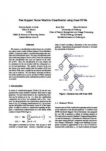
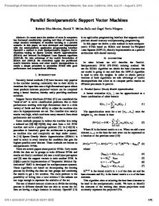
5. Performance In this section we compare the hybrid OpenMP/MPI version of our software with one using only MPI, and also our implementation against three other parallel SVM solvers. Data sets are taken from the PASCAL Challenge on Large-scale Learning, and the sizes we used are shown in Table 1. Due to memory restrictions, we reduced the number of samples in the FD and DNA data sets. Additionally, the DNA data set was modified from categories to binary features, increasing m by a factor of 4. The data sets were converted into a simple feature representation in SVM-light format. The software was run on a cluster of quad-core 3GHz Intel Xeon processors, each with 2GB RAM. The GotoBLAS library was used for BLAS functions, with the number of OpenMP threads set to 4, to match the number of cores. We also used the LAM implementation of the MPI library. To compare the hybrid approach (using the techniques described in Sections 4.1 and 4.2) with pure MPI (using Section 4.1 only), we used the data sets alpha to zeta. The results are shown in Figure 1. They consistently show that, although the pure MPI approach has better properties in terms of parallel efficiency, the hybrid approach is always computationally more efficient. We believe this is a result of the multi-core processor architecture. The cores are associated with relatively small local cache memories, and such an architecture demands a fine-grained parallelism where, to reduce bus traffic, an operation is split into tasks that operate on small portions of data (Buttari et al., 2009). OpenMP is better suited to this fine-grained parallelism. We made a comparison with other parallel software PGPDT (Zanni et al., 2006), PSVM (Chang et al., 2008), and Milde (Durdanovic et al., 2007). All of them are able to handle nonlinear as well as linear kernels, unlike our implementation. Using a linear kernel in each case, the results are shown 1945


(a)

(b)

100

10

100

10 4

8 16 Number of processor cores

32

(c)

4

32

MPI only, τ=0.01 MPI only, τ=1 MPI/OpenMP, τ=0.01 MPI/OpenMP, τ=1 Perfect parallelization

Training time (s)

1000

100

10

100

10 4


32

(e)

4


32

(f) MPI only, τ=0.01 MPI only, τ=1 MPI/OpenMP, τ=0.01 MPI/OpenMP, τ=1 Perfect parallelization Training time (s)

MPI only, τ=0.01 MPI only, τ=1 MPI/OpenMP, τ=0.01 MPI/OpenMP, τ=1 Perfect parallelization Training time (s)


(d) MPI only, τ=0.01 MPI only, τ=1 MPI/OpenMP, τ=0.01 MPI/OpenMP, τ=1 Perfect parallelization

Training time (s)


1000

Training time (s)

Training time (s)


1000

100

1000

100 8

16 Number of processor cores

32

8

16 Number of processor cores

32

Figure 1: SVM training time with respect to the number of processors, for the PASCAL data sets (a) alpha, (b) beta, (c) gamma, (d) delta, (e) epsilon and (f) zeta. For each data set we trained using two values of τ. The results show that, although the pure MPI approach shows better parallel efficiency properties, the hybrid approach is always computationally more efficient.

1946


Data Set Alpha Beta Gamma Delta Espilon Zeta FD OCR DNA

n 500000 500000 500000 500000 500000 500000 2560000 3500000 6000000

m 500 500 500 500 2000 2000 900 1156 800

Table 1: PASCAL Challenge on Large-scale Learning data sets used in this paper. Data Set

# cores

Alpha

16

Beta

16

Gamma

16

Delta

16

Epsilon

32

Zeta

32

FD

32

OCR

32

DNA

48

τ 1 0.01 1 0.01 1 0.01 1 0.01 1 0.01 1 0.01 1 0.01 1 0.01 1 0.01

OOPS 39 50 120 48 44 49 40 46 730 293 544 297 3199 2152 1361 1330 2668 6557

PGPDT 3673 4269 5003 4738 — 7915 — 9492 — — — — — — — — — —

PSVM 1684 4824 2390 4816 1685 4801 1116 4865 17436 36319 14368 37283 — — — — — —

Milde (80611) (85120) (83407) (84194) (83715) (84445) (57631) (84421) (58488) (56984) (22814) (68059) (39227) (52408) (58307) (36523) — 14821

Table 2: Comparison of parallel SVM training software on PASCAL data sets. Times are in seconds. In all cases except the DNA data set, the Milde software ran but did not terminate within 24 hours of runtime, so the numbers in brackets show when it was within 1% of its final objective value; — indicates that the software failed to load the problem.

in Table 2. With the exception of Milde (which has its own message passing implementation), the LAM implementation of the MPI library was used. We required an objective value accuracy of ε = 0.01, and chose two values for τ within the range set in the Challenge, so we believe the training tasks are representative. In keeping with the evaluation method of the Challenge, the timings shown are for training and do not include time spent reading the data. The PSVM algorithm includes an additional partial Cholesky factorization 1947


Data Set

τ n

Alpha Beta Gamma Delta Epsilon Zeta FD OCR DNA

1 0.01 1 0.01 1 0.01 1 0.01 1 0.01 1 0.01 1 0.01 1 0.01 1 0.01

Parallel OOPS cores

500,000

16

500,000

16

500,000

16

500,000

16

500,000

32

500,000

32

2,560,000

48

3,500,000

32

6,000,000

48

OOPS t 39 50 120 48 44 49 40 46 730 293 544 297 3199 2152 1361 1330 2668 6557

n 500,000 500,000 500,000 500,000 210,000 230,000 500,000 250,000 600,000

t 122 151 394 154 149 163 137 134 951 374 1115 449 1502 840 275 297 175 176

Single processor LibLinear n t 147 500,000 112 135 500,000 112 (8845) 500,000 348.33 (13266) 500,000 429 316 250,000 265 278 250,000 248 231 500,000 193 181 250,000 121 144 600,000 30

LaRank n t 3354 500,000 2474 6372 500,000 1880 — 500,000 20318 — 500,000 — 5599 500,000 2410 — 500,000 — 1537 500,000 332 5695 500,000 4266 300 600,000 407

Table 3: Comparison of our SVM training software OOPS, in parallel and on a single processor, with linear SVM software LibLinear and LaRank, again on PASCAL data sets. Times for training are in seconds. For the parallel software OOPS, each core had access to 2GB memory. The single processor codes had access to 4 cores and 8GB memory, and the larger data sets were reduced in size to fit. For LibLinear, brackets indicate that the iteration limit was reached. For LaRank, — indicates that the software did not terminate within 24 hours. Data Set Alpha Beta Gamma Delta Epsilon Zeta FD OCR

OOPS 0.1345 0.4988 0.1174 0.1344 0.0341 0.0115 0.2274 0.1595

LibLinear 0.1601 0.4988 0.1185 0.1346 0.4935 0.4931 0.2654 0.1660

LaRank 0.1606 0.5001 0.1187 0.1355 0.4913 0.4875 0.3081 0.1681

Table 4: Accuracy measured using area under precision recall curve. These values are taken from the test results tables of the Evaluation pages of the PASCAL Challenge website.

procedure, which we also do not include in the training times. To make the training equivalent, the rank of the factorization was set to be the number of features m. The Milde software includes a number of termination criteria but not one based on the objective. Using the default criteria of maximum gradient below ε resulted in the software never terminating in all but one case within a 24 1948


hour runtime limit. To be closer to the spirit of the Challenge, we show the time taken to be within 1% of the objective value at the end of 24 hours when the program was terminated prematurely, although in many cases the output indicated that the method was not yet converging. The results show that our approach described in this paper and implemented in OOPS is typically one to two orders of magnitude faster than the other parallel SVM solvers, terminates reliably, and training times are reasonably consistent for different values of τ. Unfortunately there were no other linear SVM implementations in the Parallel track of the PASCAL Challenge. Instead, we show in Table 3 training time results for two linear SVM codes that did participate in the PASCAL Challenge: LibLinear (Fan et al., 2008) which won the linear SVM track, and LaRank (Bordes et al., 2007) specialised for linear SVMs. Both codes ran serially, using the memory of 4 processor cores (8GB RAM in total), although it should be noted that as we used the GotoBLAS library when building LibLinear, it was able to use all four processor cores during BLAS operations. To make training possible, it was necessary to reduce the size of the larger data sets from the sizes given in Table 1; the number of samples used each time are shown as n in Table 3. The presentation of the results is slightly unusual in that training times are not directly connected to accuracy results against a test set. This is because labelled validation and test data sets have not been made publicly available. Performance statistics related to the precision recall curve were evaluated on the Challenge website, and so instead we reproduce in Table 4 the results from the website for area under the precision recall curve results for the test data set. In general the precision of our method is consistent with the best of the other linear SVM methods that participated. Taking the results in Tables 3 and 4 together, it is clear that LibLinear in particular is a very efficient implementation, even in the cases Alpha to Delta where it is working with the full data set. Table 4 clearly indicates that our approach consistently finds a high-quality solution to the separating hyperplane, measured in terms of classification accuracy, whereas for LibLinear the quality of the solution is lower. In many cases, the reduction in prediction accuracy is only small. The results in Table 4 for the Epsilon and Zeta data sets in particular show, however, that for some problems the quality of the solution from OOPS can be substantially better.

6. Conclusions In this paper, we have shown how to develop a hybrid parallel implementation of linear Support Vector Machine training. The approach allows the entire data set to be used, and consists of the following steps: 1. Reformulating the problem to remove the dense Hessian matrix. 2. Using interior point method to solve the optimization problem in a predictable time, and Cholesky decomposition to give good numerical stability of implicit inverses. 3. Exploiting the block structure of the augmented system matrix, to partition the data and linear algebra computations amongst parallel processing nodes efficiently. 4. Within SMP nodes, casting the main computations as matrix-matrix multiplication where possible, partitioning the matrices to obtain better data locality, and using highly efficient BLAS implementation for a multi-threaded architecture. The above steps were implemented in OOPS. Our results show that, for all cases, the hybrid implementation was faster than one using purely MPI, even though the MPI version had better parallel 1949


efficiency. We used the hybrid implementation to solve very large problems from the PASCAL Challenge on Large-scale Learning, of up to a few million data samples. On these problems the approach described in this paper was highly competitive, and showed that even on data sets of this size, training times in the order of minutes are possible. In this paper we have focused on linear kernels. It is possible to extend the techniques described above to handle non-linear kernels, by approximating the positive semidefinite kernel matrix K with a low-rank outer product representation such as partial Cholesky factorization LLT ≈ K (Fine and Scheinberg, 2002). This approach produces the first r columns of the matrix L (corresponding to the r largest pivots) and leaves the other columns as zero, giving an approximation of the matrix K of rank r. Extending the work of Fine and Scheinberg, the diagonal D ∈ Rn×n of the residual matrix (K − LLT ) can be determined at no extra expense and included in a separable formulation for non-linear kernels: 1 T min (w w + zT Dz) − eT z w,z 2 s.t. w − (Y L)T z = 0 − yT z = 0 0 ≤ z ≤ τe. Chang et al. (2008) describe how to perform partial Cholesky decomposition in a parallel environment. Data is segmented between the processors. All diagonal elements are calculated to determine pivot candidates. Then, for each of the r columns, the largest diagonal element is located. The corresponding pivot row of L and the original features need to be known by all processors, so this information is broadcast by the owner processor. With this information, all processors can update the section of the new column of L for which they are responsible, and also update corresponding diagonal elements. Although the algorithm requires the processors to be synchronised at each iteration, little of the data needs to be shared amongst the processors: the bulk of the communication between processors is limited to a vector of length m and a vector of at most length r. Note that matrix K is known only implicitly, through the kernel function, and calculating its values is an expensive process. The algorithm therefore calculates each kernel element required to form L only once, giving a complexity of O (nr2 + nmr) for the initial Cholesky factorization, and O (nr2 + r3 ) for each IPM iteration of our algorithm. The method described in this paper requires all sample data to be loaded into memory, and this clearly has an impact on the size of problem that can be tackled. It is possible to improve data handling and increase the storage capacity somewhat, for instance storing the data compactly and expanding sections into floating point numbers when needed by the BLAS routines (Durdanovic et al., 2007), but the scaling is still O (nm2 ). The direction of our further research is to develop methods that are able to safely ignore or remove data points from consideration as the algorithm progresses. In conjunction with exploiting the structure of the optimization problem as described in this paper, we believe this will offer further significant improvements to the overall training time.

Acknowledgments The authors would like to thank the PASCAL organisers for the Challenge, the anonymous referees for their comments, Professor Zanni for providing the PGPDT software, and Dr Durdanovic for assistance with the Milde software. This work has made use of the resources provided by the 1950


Edinburgh Compute and Data Facility (ECDF, http://www.ecdf.ed.ac.uk/). The ECDF is partially supported by the eDIKT initiative (http://www.edikt.org).

References Antoine Bordes, Léon Bottou, Patrick Gallinari, and Jason Weston. Solving multiclass support vector machines with LaRank. In Zoubin Ghahramani, editor, Proceedings of the 24th International Machine Learning Conference, pages 89–96, Corvallis, Oregon, 2007. OmniPress. URL http://leon.bottou.org/papers/bordes-2007. Alfredo Buttari, Julien Langou, Jakub Kurzak, and Jack Dongarra. A class of parallel tiled linear algebra algorithms for multicore architectures. Parallel Computing, 35(1):38–53, January 2009. Edward Chang, Kaihua Zhu, Hao Wang, Hongjie Bai, Jian Li, Zhihuan Qiu, and Hang Cui. Parallelizing support vector machines on distributed computers. In J.C. Platt, D. Koller, Y. Singer, and S. Roweis, editors, Advances in Neural Information Processing Systems 20, pages 257–264, Cambridge, MA, 2008. MIT Press. Ronan Collobert, Samy Bengio, and Yoshua Bengio. A parallel mixture of SVMs for very large scale problems. Neural Computation, 14(5):1105–1114, 2002. Jian-xiong Dong, Adam Krzyzak, and Ching Suen. A fast parallel optimization for training support vector machine. In P. Perner and A. Rosenfeld, editors, Proceedings of 3rd International Conference on Machine Learning and Data Mining, pages 96–105, Leipzig, Germany, 2003. Springer Lecture Notes in Artificial Intelligence. Igor Durdanovic, Eric Cosatto, and Hans-Peter Graf. Large scale parallel SVM implementation. In Léon Bottou, Olivier Chapelle, Dennis DeCoste, and Jason Weston, editors, Large Scale Kernel Machines, chapter 5, pages 105–38. MIT Press, 2007. Rong-En Fan, Kai-Wei Chang, Cho-Jui Hsieh, Xiang-Rui Wang, and Chih-Jen Lin. LIBLINEAR: A library for large linear classification. Journal of Machine Learning Research, 9:1871–1874, 2008. Michael Ferris and Todd Munson. Interior point methods for massive support vector machines. SIAM Journal on Optimization, 13(3):783–804, 2003. Shai Fine and Katya Scheinberg. Efficient SVM training using low-rank kernel representations. Journal of Machine Learning Research, 2:243–264, 2002. Glenn Fung and Olvi L. Mangasarian. Proximal support vector machine classifiers. In F. Provost and R. Srikant, editors, Proceedings KDD-2001: Knowledge Discovery and Data Mining, August 26-29, 2001, San Francisco, CA, pages 77–86, New York, 2001. Asscociation for Computing Machinery. Jacek Gondzio and Andreas Grothey. Parallel interior point solver for structured quadratic programs: Application to financial planning problems. Annals of Operations Research, 152(1): 319–339, 2007. 1951


Jacek Gondzio and Robert Sarkissian. Parallel interior point solver for structured linear programs. Mathematical Programming, 96(3):561–584, 2003. Kazushige Goto and Robert A. van de Geijn. Anatomy of high-performance matrix multiplication. ACM Trans. Math. Softw., 34(3):1–25, 2008. Hans Peter Graf, Eric Cosatto, Léon Bottou, Igor Dourdanovic, and Vladimir Vapnik. Parallel support vector machines: the Cascade SVM. In Lawrence Saul, Yair Weiss, and Léon Bottou, editors, Advances in Neural Information Processing Systems. MIT Press, 2005. volume 17. José R. Herrero. A Framework for Efficient Execution of Matrix Computations. PhD thesis, Universitat Politècnica de Catalunya (UPC), July 2006. Bo K˚agström, Per Ling, and Charles van Loan. GEMM-based level 3 BLAS: high-performance model implementations and performance evaluation benchmark. ACM Trans. Math. Softw., 24 (3):268–302, 1998. Glenn R. Luecke, Jae H. Yun, and Philip W. Smith. Performance of parallel cholesky factorization algorithms using blas. The Journal of Supercomputing, 6(3):315–329, December 1992. MPI-Forum. MPI: A Message-Passing Interface Standard. University of Tennessee, Knoxville, Tennessee, 1.1 edition, June 1995. URL http://www.mpi-forum.org. OpenMP Architecture Review Board. OpenMP Application Program Interface, 3.0 edition, May 2008. URL http://www.openmp.org. Edgar Osuna, Robert Freund, and Federico Girosi. An improved training algorithm for support vector machines. In J. Principe, L. Gile, N. Morgan, and E. Wilson, editors, Neural Networks for Signal Processing VII — Proceedings of the 1997 IEEE Workshop, pages 276–285. IEEE, 1997. John Platt. Fast training of support vector machines using sequential minimal optimization. In Bernhard Schölkopf, Christopher. J. C. Burges, and Alexander. J. Smola, editors, Advances in Kernel Methods: Support Vector Learning, pages 185–208. MIT Press, 1999. Rolf Rabenseifner and Gerhard Wellein. Comparison of parallel programming models on clusters of SMP nodes. In Hans Georg Bock, Ekaterina Kostina, Hoang Xuan Phu, and Rolf Rannacher, editors, Modelling, Simulation and Optimization of Complex Processes: Proceedings of the International Conference on High Performance Scientific Computing, March 10-14, 2003, Hanoi, Vietnam, pages 409–426. Springer, 2003. Lorna Smith and Mark Bull. Development of mixed mode MPI / OpenMP applications. Scientific Programming, 2001. Soeren Sonnenburg, Vojtech Franc, Elad Yom-Tov, and Michele Sebag. PASCAL large scale learning challenge, 2008. URL http://largescale.first.fraunhofer.de/. Amund Tveit and Havard Engum. Parallelization of the incremental proximal support vector machine classifier using a heap-based tree topology. Technical report, IDI, NTNU, Trondheim, 2003. 1952


Vladimir Vapnik. Statistical Learning Theory. Wiley, 1998. Kristian Woodsend and Jacek Gondzio. Exploiting separability in large-scale support vector machine training. Technical Report MS-07-002, School of Mathematics, University of Edinburgh, August 2007. Submitted for publication. Available at http://www.maths.ed.ac.uk/ ˜gondzio/reports/wgSVM.html. Stephen J. Wright. Primal-Dual Interior-Point Methods. S.I.A.M., 1997. Gaetano Zanghirati and Luca Zanni. A parallel solver for large quadratic programs in training support vector machines. Parallel Computing, 29(4):535–551, 2003. Luca Zanni, Thomas Serafini, and Gaetano Zanghirati. Parallel software for training large scale support vector machines on multiprocessor systems. Journal of Machine Learning Research, 7: 1467–1492, 2006.

1953