E-mail: [duch,raad,kgrabcze]@phys.uni.torun.pl. May 18, 2000. Abstract. Methodology of extraction of optimal sets of logical rules using neural networks and ...
Hybrid neural-global minimization method of logical rule extraction ˙ Włodzisław Duch, Rafał Adamczak, Krzysztof Gra¸bczewski and Grzegorz Zal Department of Computer Methods, Nicholas Copernicus University, Grudzia¸dzka 5, 87-100 Toru´n, Poland. E-mail: [duch,raad,kgrabcze]@phys.uni.torun.pl May 18, 2000
Abstract Methodology of extraction of optimal sets of logical rules using neural networks and global minimization procedures has been developed. Initial rules are extracted using density estimation neural networks with rectangular functions or multi-layered perceptron (MLP) networks trained with constrained backpropagation algorithm, transforming MLPs into simpler networks performing logical functions. A constructive algorithm called C-MLP2LN is proposed, in which rules of increasing specificity are generated consecutively by adding more nodes to the network. Neural rule extraction is followed by optimization of rules using global minimization techniques. Estimation of confidence of various sets of rules is discussed. The hybrid approach to rule extraction has been applied to a number of benchmark and real life problems with very good results. Keywords: computational intelligence, neural networks, extraction of logical rules, data mining
1
Logical rules - introduction.
Why should one use logical rules if other methods of classification – machine learning, pattern recognition or neural networks – may be easier to use and give better results? Adaptive systems M W , including the most popular neural network models, are useful classifiers that adjust internal parameters W performing vector mappings from the input to the output space. Although they may achieve high accuracy of classification the knowledge acquired by such systems is represented in a set of numerical parameters and architectures of networks in an incomprehensible way. Logical rules should be preferred over other methods of classification provided that the set of rules is not too complex and classification accuracy is sufficiently high. Surprisingly, in many applications simple rules proved to be more accurate and were
able to generalize better than various machine and neural learning algorithms. Many statistical, pattern recognition and machine learning [1] methods of finding logical rules have been designed in the past. Neural networks are also used to extract logical rules and select classification features. Unfortunately systematic comparison of neural and machine learning methods is still missing. Many neural rule extraction methods have recently been reviewed and compared experimentally [2], therefore we will not discuss them here. Neural methods focus on analysis of parameters (weights and biases) of trained networks, trying to achieve high fidelity of performance, i.e. similar results of classification by extracted logical rules and by the original networks. Non-standard form of rules, such as M -of-N rules (M out of N antecedents should be true), fuzzy rules, or decision trees [1] are sometimes useful but in this paper we will consider only standard IF ... THEN propositional rules. In classification problems propositional rules may take several forms. Very general form of such rule is: IF X ∈ K (i) THEN Class(X) = Ci , i.e. if X belongs to the cluster K (i) then its class is Ci =Class(K (i) ), the same as for all vectors in this cluster. If clusters overlap non-zero probability of classification p(C i |X; M ) for several classes is obtained. This approach does not restrict the shapes of clusters used in logical rules, but unless the clusters are visualized in some way (a difficult task in highly dimensional feature spaces) it does not give more understanding of the data than any black box classifier. A popular simplification of the most general form of logical rules is to describe clusters using separable “membership” functions. This leads to fuzzy rules, for example in the form: µ(k) (X) p(Ck |X; M ) = � (i) i µ (X) where µ(k) (X) =
� i
(k)
µi (Xi )
(1)
(2)
Journal of Advanced Computational Intelligence Vol. 3, 1999
and µ(k) (X) is the value of the membership function defined for cluster k. Such context-dependent or clusterdependent membership functions are used in the Feature Space Mapping (FSM) neurofuzzy system [3]. The flexibility of this approach depends on the choice of membership functions. Fuzzy logic classifiers use most frequently a few triangular membership functions per one input feature [4]. These functions do not depend on the region of the input space, providing oval decision borders, similar to Gaussian functions (cf. Fig.1). Thus fuzzy rules give decision borders that are not much more flexible than those of crisp rules. More important than softer decision borders is the ability to deal with oblique distribution of data by rotating some decision borders. This requires new linguistic variables formed by taking linear combination or making non-linear transformations of input features, but the meaning of such rules is sometimes difficult to comprehend (cf. proverbial “mixing apples with oranges”). Logical rules require symbolic inputs (linguistic variables), therefore the input data has to be quantized first, i.e. the features defining the problem should be identified and their values (sets of symbolic or integer values, or continuous intervals) labeled. For example a variable “size” will have the value “small” if the continuous variable x k measuring size falls in some specified range, xk ∈ [a, b]. Using one input variable several binary (logical) variables may be created, for example s1 = δ(size, small) equal to 1 (true) only if variable “size” has the value “small”. The rough set theory [5] is used to derive crisp logic propositional rules. In this theory for two-class problems the lower approximation of the data is defined as a set of vectors or a region of the feature space containing input vectors that belong to a single class with probability = 1, while the upper approximation covers all instances which have a chance to belong to this class (i.e. probability is > 0). In practice the shape of the boundary between the upper and the lower approximations depends on the indiscernibility (or similarity) relation used. Linear approximation to the boundary region leads to trapezoidal membership functions. The simplest crisp form of logical rules is obtained if trapezoidal membership functions are changed into rectangular functions. Rectangles allow to define logical linguistic variables for each feature by intervals or sets of nominal values. A fruitful way of looking at logical rules is to treat them as an approximation to the posterior probability of classification p(Ci |X; M ), where the model M is composed of the set of rules. Crisp, fuzzy and rough set decision borders are a special case of the FSM neurofuzzy approach [3] based on separable functions used to estimate the classification probability. Although the decision borders of crisp logical rule classification are much simpler than those achievable by neural networks, results
2
2
1.5
1
0.5
0
2
2
1.5
1.5
1
1
0.5
0.5
0
0
0.5
1
1.5
2
0
0.5
1
1.5
2
0 0
0.5
1
1.5
2
Figure 1: Shapes of decision borders for general clusters, fuzzy rules (using product of membership function), rough rules (trapezoidal approximation) and logical rules. are sometimes significantly better. Three possible explanations of this empirical observation are: 1) the inability of soft sigmoidal functions to represent sharp, rectangular edges that may be necessary to separate two classes, 2) the problem of finding globally optimal solution of the non-linear optimization problem for neural classifiers – since we use a global optimization method to improve our rules there is a chance of finding a better solution than gradient-based neural classifiers are able to find; 3) the problem of finding an optimal balance between the flexibility of adaptive models and the danger of overfitting the data. Although Bayesian regularization [6] may help in case of some neural and statistical classification models, logical rules give much better control over the complexity of the data representation and elimination of outliers. We are sure that in all cases, independently of the final classifier used, it is advantageous to extract crisp logical rules. First, in our tests logical rules proved to be highly accurate; second, they are easily understandable by experts in a given domain; third, they may expose problems with the data itself. This became evident in the case of the “Hepar dataset”, collected by dr. H. Wasyluk and co-workers from the Postgraduate Medical Center in Warsaw. The data contained 570 cases described by 119 values of medical tests and other features and were collected over a period of more than 5 years. These cases were divided into 16 classes, corresponding to different types of liver disease (final diagnosis was confirmed by analysis of liver samples under microscope, a procedure that we try to avoid by providing reliable diagnosis system). We have extracted crisp logical rules from this dataset using our C-MLP2LN approach described below, and found that 6 very simple rules gave 98.5% accuracy.
Journal of Advanced Computational Intelligence Vol. 3, 1999
Unfortunately these rules also revealed that the missing attributes in the data were replaced by the averages for a given class, for example, cirrhosis was fully characterized by the rule “feature 5=4.39”. Although one may report very good results using crossvalidation tests using this data, such data is of course useless since the averages for a given class are known only after the diagnosis. In this paper a new methodology for logical rule extraction is presented, based on constructive MLPs for initial feature selection and rule extraction, and followed by rule optimization using global minimization methods. This approach is presented in detail in the next section and illustrative applications to a few benchmark problems are given in the third section. The fourth section contains applications to a real life medical data. The paper is finished with a short discussion.
2
The hybrid methodology
rule
extraction
Selection of initial linguistic variables (symbolic inputs) is the first step of the rule extraction process. Linguistic variables are optimized together with rules in an iterative process: neural networks with linguistic inputs are constructed, analysed, logical rules are extracted, intervals defining linguistic variables are optimized using rules, and the whole process repeated until convergence is achieved (usually two or three steps are sufficient, depending on the initial choice). Linguistic (logical) input variables s k , for integer or symbolic variables xi , taking values from a finite set of (j) elements Xi = {Xi }, are defined as true if x i belongs to a specific subset Xik ⊆ Xi . Defining X as a subset of integers such linguistic variables as “prime-number” or “odd-number” may be defined. For continuous input features xi linguistic variable s k is obtained by specifying an open or closed interval x i ∈ [Xk , Xk� ] or some other predicate P k (xi ). Each continuous input feature xi is thus replaced by two or more linguistic values for which predicates Pk are true or false. For neural networks a convenient representation of these linguistic values is obtained using vectors of predicates, for example Vs1 = (+1, −1, −1...) for linguistic variable s 1 or Vs2 = (−1, +1, −1...) for s2 etc. Initial values of the intervals for continuous linguistic variables may be determined by the analysis of histograms, dendrograms, decision trees or clusterization methods. Neural-based methods are also suitable to select relevant features and provide initial intervals defining linguistic variables. FSM, our density estimation neurofuzzy network, is initialized using simple clusterization methods [7], for example dendrogram analysis of the input data vectors (for very large datasets rounding
3
of continuous values to lower precision is applied first, and then duplicate data vectors are sorted out to reduce the number of input vectors). Rectangular functions may be used in FSM for a direct extraction of logical rules. MLP (multilayered perceptron) neural models may find linguistic variables by training a special neural layer [8] of L-units (linguistic units). Each L-unit is a combination of two sigmoidal functions realizing the function L(xi ; bi , b�i , β) = σ(β(xi − bi )) − σ(β(xi − b�i )), parameterized by two biases b, b � determining the interval in which this function has non-zero value. The slope β of sigmoidal functions σ(βx) is slowly increased during the learning process, transforming the fuzzy membership function (“soft trapezoid”) into a window-type rectangular function [3, 8] (for simplicity of notation the dependence of L-functions on the slope is not shown below). Similar smooth transformation is used in the FSM network using biradial transfer functions, which are combinations of products of L(x i ; bi , b�i ) functions [9] with some additional parameters. Outputs of L-units filtered through L(xi ; bi , b�i ) are usually � combined and � another sigmoid σ( L(x ; b , b )) or the product i ij ij ij � � ij L(xi ; bij , bij )) of these functions is used.
+1
b
W
x
1
W2
σ(W x+b) 1
+1
b
b'
b
b'
-1 σ(W x+b') 2
+1 b'
Figure 2: L-units, or pairs of neurons with constrained weights, used for determination of linguistic variables. After initial definition of linguistic variables neural network is constructed and trained. To facilitate extraction of logical rules from an MLP network one should transform it smoothly into something resembling a network performing logical operations (Logical Network, LN). This transformation, called MLP2LN [10], may be realized in several ways. Skeletonization of a large MLP network is the method of choice if our goal is to find logical rules for an already trained network. Otherwise it is simpler to start from a single neuron and construct the logical network using the training data. Since interpretation of the activation of the MLP network nodes is not easy [11] a smooth transition from MLP to a logical-type of network performing similar functions is advocated. This is achieved by: a) gradually increasing the slope β of sigmoidal functions to obtain crisp decision regions; b) simplifying the network structure by inducing the weight decay through a penalty term; c) enforcing the integer weight values 0 and ±1, interpreted
Journal of Advanced Computational Intelligence Vol. 3, 1999
4
as 0 = irrelevant input, +1 = positive and −1 = negative evidence. These objectives are achieved by adding two additional terms to the standard mean square error function E0 (W ):
the simplicity/accuracy tradeoff of the generated network and extracted rules. If a very simple network (and later logical rules) is desired, giving only rough description of the data, λ1 should be as large as possible: although one may estimate the relative size of the regularization term (3) versus the mean square error (MSE) a few experiments E(W ) = E0 (W ) + are sufficient to find the largest value for which the MSE λ1 � 2 λ2 � 2 Wij + W (Wij − 1)2 (Wij + 1)2 is still acceptable and does not decrease quickly when 2 i,j 2 i,j ij λ1 is decreased. Smaller values of λ 1 should be used to The first term, scaled by the λ 1 hyperparameter, en- obtain more accurate networks (rules). The value of λ 2 courages weight decay, leading to skeletonization of the should reach the value of λ 1 near the end of the training. network and elimination of irrelevant features. The secLogical rule extraction: the slopes of sigmoidal ond term, scaled by λ 2 , forces the remaining weights to functions are gradually increased to obtain sharp deciapproach ±1, facilitating easy logical interpretation of sion boundaries and the complex decision regions are the network function. In the backpropagation training transformed into simpler, hypercuboidal decision realgorithm these new terms lead to the additional change gions. Rules R implemented by trained networks are k of weights: λ1 Wij + λ2 Wij (Wij2 − 1)(3Wij2 − 1). The obtained in the form of logical conditions by considerlast, 6-th order regularization term in the cost function, ing contributions of inputs for each linguistic variable s, may be replaced by one of the lower order terms: represented by a vector V . Contribution of variable s to s
|Wij ||Wij2 − 1| cubic |Wij | + +1 �
|Wij2
(4)
− 1| quadratic
1 1 |Wij + k| − |Wij − | − |Wij + | − 1 2 2
the activation is equal to the dot product V s · Ws of the subset Ws of the weight vector corresponding to the V s inputs. A combination of linguistic variables activating the hidden neuron above the threshold is a logical rule of the form: R= (s1 ∧ ¬s2 ∧ ... ∧ sk ).
In the constructive version of the MLP2LN approach (called C-MLP2LN) usually one hidden neuron per outIntroduction of integer weights may also be justified put class is created at a time and the training proceeds from the Bayesian perspective [6]. The cost function until the modified cost function reaches minimum. The specifies our prior knowledge about the probability disweights and the threshold obtained are then analyzed tribution P (W |M ) of the weights in our model M . For and the first group of logical rules is found, covering classification task when crisp logical decisions are rethe most common input-output relations. The input data quired the prior probability of the weight values should that are correctly handled by the first group of neurons include not only small weights but also large positive and will not contribute to the error function, therefore the negative weights distributed around ±1, for example: weights of these neurons are kept frozen during further (5) training. This is equivalent to training one neuron (per P (W |M ) = Z(α)−1 e−αE(W |M) ∝ � � class) at a time on the remaining data, although some2 2 e−α1 Wij e−α2 |Wij −1| times training two or more neurons may lead to faster ij ij convergence. This procedure is repeated until all the where the parameters α i play similar role for proba- data are correctly classified, weights analyzed and a set bilities as the parameters λi for the cost function. Using of rules R1 ∨ R2 ...∨ Rn is found for each output class alternative cost functions amounts to different priors for or until the number of rules starts to grow rapidly. The regularization, for example Laplace instead of Gaussian output neuron for a given class is connected to the hidden prior. Initial knowledge about the problem may also be neurons created for that class – in simple cases only one inserted directly into the network structure, defining ini- neuron may be sufficient to learn all instances, becoming tial conditions modified further in view of the incoming an output neuron rather than a hidden neuron. Output data. Since the final network structure becomes quite neurons perform simple summation of the hidden nodes simple insertion of partially correct rules to be refined by signals. Since each time only one neuron per class is the learning process is quite straightforward. trained the C-MLP2LN training is fast. The network reAlthough constraints Eq. (3) do not change the MLP peatedly grows when new neurons are added, and then exactly into a logical network they are sufficient to fa- shrinks when connections are deleted. Since the first cilitate logical interpretation of the final network func- neuron for a given class is trained on all data for that tion. MLPs are trained using relatively large λ 1 value class the rules it learns are most general, covering largest at the beginning, followed by a large λ 2 value near the number of instances. Therefore rules obtained by this alend of the training process. These parameters determine gorithm are ordered, starting with rules that cover many k=−1
Journal of Advanced Computational Intelligence Vol. 3, 1999
5
training set. Changing the value of λ 1 will produce a series of models with higher and higher confidence of correct classification at the expense of growing rejection rate. A set of rules may classify some cases at the 100% confidence level; if some instances are not covered by this set of rules another set of (usually simpler) rules at a lower confidence level is used (confidence level is estimated as the accuracy of rules achieved on the training set). In this way a reliable estimation of confidence is possible. The usual procedure is to give only one set of rules, assigning to each rule a�confidence factor, for example ci = P (Ci , Ci |M )/ j P (Ci , Cj |M ). This is rather misleading. A rule R (1) that does not make any errors covers typical instances and its reliability is close to 100%. If a less accurate rule R (2) is given, for example classifying correctly 90% of instances, the reliability of classification for instances covered by the first rule is still close to 100% and the reliability of classification in the border region (R (2) \R(1) , or cases covered by R(2) but not by R(1) ) is much less than 90%. Including just these border cases gives much lower confidence M factors and since the number of such cases is relatively over all parameters M , or minimizing the number small the estimate itself has low reliability. A possibility of wrong predictions (possibly with some risk matrix sometimes worth considering is to use a similarity-based R(Ci , Cj )): classifier (such as the k-NN method or RBF network) to � improve accuracy in the border region. min R(Ci , Cj )P(Ci , Cj |M ) (7) Logical rules, similarly as any other classification sysM i�=j tems, may become brittle if the decision borders are Weighted combination of these two terms: placed too close to the data vectors instead of being � placed between the clusters. The brittleness problem P(Ci , Cj |M ) − Tr P(Ci , Cj |M ) (8) E(M ) = λ is solved either at the optimization stage by selecting i�=j the middle values of the intervals for which best perforis bounded by −n and should be minimized over pa- mance is obtained or, in a more general way, by adding rameters M without constraints. For this minimiza- noise to the data [13]. So far we have used the first tion we have used simulated annealing or multisimplex method: starting from the values of the optimized paramglobal minimization methods. If λ is large the number eters the largest cuboid in the parameter space in which of errors after minimization may become zero but some the number of errors is constant is determined. The ceninstances may be rejected (i.e. rules will not cover the ter of this cuboid is taken as the final estimation of the whole input space). Since rules discriminate between in- adaptive parameters. stances of one class and all other classes one can define a cost function for each rule separately:
cases and ending with rules that cover only a few cases. Simplification of rules: the final solution may be presented as a set of logical rules or as a network of nodes performing logical functions. However, some rules obtained from analysis of the network may involve spurious conditions, more specific rules may be contained in general rules or logical expressions may be simplified if written in another form. Therefore after extraction rules are carefully analyzed and whenever possible simplified (we use a Prolog program for this step). Optimization of rules: optimal intervals and other adaptive parameters may be found by maximization of a predictive power of a classifier. Let P(C i , Cj |M ) be the confusion matrix, i.e. the number of instances in which class Cj is predicted when the true class was Ci , given some parameters M . Then for n samples p(Ci , Cj |M ) = P(Ci , Cj |M )/n is the probability of (mis)classification. The best parameters M are selected by maximizing the number (or probability) of correct predictions (called also the “predictive power” of rules): (6) max [Tr P(Ci , Cj |M )]
ER (M ) = λ(P+− + P−+ ) − (P++ + P−− )
(9)
and minimize it over parameters M used in the rule R only (+ means here one of the classes, and − means all other classes). The combination P ++ /(P++ + P+− ) ∈ (0, 1] is sometimes called the sensitivity of a rule [12], while P−− /(P−− + P−+ ) is called the specificity of a rule. Some rule induction methods optimize such combinations of Px,y values. Estimation of the accuracy of rules is very important, especially in medicine. Tests of classification accuracy should be performed using stratified 10-fold crossvalidation, each time including rule optimization on the
3
Illustrative benchmark applications.
Datasets for benchmark applications were taken from the UCI machine learning repository [14]. Application of the constructive C-MLP2LN approach to the classical Iris dataset was already presented in detail [15], therefore only new aspects related to the hybrid method are discussed here. The Iris data has 150 vectors evenly distributed in three classes: iris-setosa, iris-versicolor and iris-virginica. Each vector has 4 features: sepal length x1 and width x2 , and petal length x 3 and width x4 (all in cm). Analysis of smoothed histograms (assuming Gaus-
Journal of Advanced Computational Intelligence Vol. 3, 1999
sian width for each value) of the individual features for each class provides initial linguistic variables. Assuming at most 3 linguistic variables per input feature a network with 12 binary inputs equal to ±1 (features present or absent) is constructed. For example, the medium value of a single feature is coded by (−1, +1, −1) vector. For the Iris dataset a single neuron per one class was sufficient to train the network, therefore the final network structure (Fig. 3) has 12 input nodes and 3 output nodes (hidden nodes are only needed when more than one neuron is necessary to cover all the rules for a given class). The constraint hyperparameters were increased from λ1 = 0.001 at the beginning of the training to about λ1 = 0.1 near the end, with λ 2 increasing from 0 to 0.1 to enforce integer weights near the end of the training. On average the network needed about 1000 epochs for convergence. The final weights are taken to be exactly ±1 or 0 while the final value of the slopes of sigmoids reaches 300. Using L-units with initial linguistic variables provided by the histograms very simple networks were created, with non-zero weights for only one attribute, petal length x 3 . Two rules and else condition, giving overall 95.3% accuracy (7 errors) are obtained: (1) (100%), R1 : iris-setosa if x3 < 2.5 (1) (92%), R2 : iris-virginica if x3 > 4.8 (1) (94%) R3 : else iris-versicolor The first rule is accurate in 100% of cases since the setosa class is easily separated from the two other classes. Lowering the final hyperparameters leads to the following weights and thresholds (only the signs of the weights are written): Setosa Versicolor Virginica
(0,0,0 (0,0,0 (0,0,0
0,0,0 0,0,0 0,0,0
+,0,0 0,+,-,-,+
+,0,0) 0,+,-) -,-,+)
θ=1 θ=3 θ=2
Interpretation of these weights and the resulting network function (Fig. 3) is quite simple. Only two features, x3 and x4 , are relevant and a single rule per class is found: (100%) setosa if (x3 < 2.9 ∨ x4 < 0.9) versicolor if (x3 ∈ [2.9, 4.95] ∧ x4 ∈ [0.9, 1.65]) (100%) (94%) virginica if (x3 > 4.95) ∨ (x4 > 1.65) This R(2) level set of rules allows for correct classification of 147 vectors, achieving overall 98.0% accuracy. However, the first two rules have 100% reliability while all errors are due to the third rule, covering 53 cases. Decreasing constraint hyperparameters further allows to replace one of these rules by four rules, with a total of three attributes and 11 antecedents, necessary to classify correctly a single additional vector, a clear indication that overfitting occurs. The third set of rules R (3) has been found after optimization with increasing λ (Eq. 8), reliable in 100% but
6
input
X1 X2
linguistic variables
hidden layer
s m l
l1
s m l
X3
s m l
X4
s m l
l2
l3
output
Setosa 50 cases, all correct Versicolor, 47 cases, all correct Virginica 53 cases 3 wrong
Figure 3: Final structure of the network for the Iris problem. rejecting 11 vectors, 8 virginica and 3 versicolor: (100%) setosa if (x3 < 2.9) versicolor if (x3 ∈ [2.9, 4.9] ∧ x4 < 1.7) (100%) virginica if (x3 ≥ 5.3 ∨ x4 ≥ 1.9) (100%) The reliability of classification for the 11 vectors in the border region (R (2) \ R(3) ) is rather low: with p = 8/11 they should be assigned to the virginica class and with p = 3/11 to the versicolor class. It is possible to generate more specific rules, including more features, just for the border region, or to use in this region similarity-based classification system, such as k-NN, but for this small dataset we do not expect any real improvement since the true probability distributions of leave’s sizes for the two classes of iris flowers clearly overlap. In the mushroom problem [2, 14] the database consists of 8124 vectors, each with 22 discrete attributes with up to 10 different values. 51.8% of the cases represent edible, and the rest non-edible (mostly poisonous) mushrooms. A single neuron is capable of learning all the training samples (the problem is linearly separable), but the resulting network has many nonzero weights and is difficult to analyze from the logical point of view. Using the C-MLP2LN algorithm with the cost function Eq. (3) the following disjunctive rules for poisonous mushrooms have been discovered: R1 ) odor=¬(almond∨anise∨none) R2 ) spore-print-color=green R3 ) odor=none∧stalk-surface-below-ring=scaly∧ (stalk-color-above-ring=¬brown) R4 ) habitat=leaves∧cap-color=white Rule R1 misses 120 poisonous cases (98.52% accuracy), adding rule R 2 leaves 48 errors (99.41% accuracy), adding third rule leaves only 8 errors (99.90% accuracy), and all rules R 1 to R4 classify all poisonous cases correctly. The first two rules are realized by one neuron. For large value of the weight-decay parameter
Journal of Advanced Computational Intelligence Vol. 3, 1999
only one rule with odor attribute is obtained, while for smaller hyperparameter values a second attribute (sporeprint-color) is left. Adding a second neuron and training it on the remaining cases generates two additional rules, R3 handling 40 cases and R 4 handling only 8 cases. We have also derived the same rules using only 10% of all data for training. This is the simplest systematic logical description of the mushroom dataset that we know of (some of these rules have probably been also found by the RULEX and TREX algorithms [2]) and therefore should be used as a benchmark for other rule extraction methods. We have also solved the three monk problems [16]. For the Monk 1 problem a total of 4 rules and one exception classifying the data without any errors was created (exceptions are additional rules handling patterns that are not recognized properly by the rules). In the Monk 2 problem perfect classification with 16 rules and 8 exceptions extracted from the resulting network has been achieved. The number of atomic formulae which compose them is 132. In the Monk 3 problem, although the training data for this problem is corrupted by 5% noise it is still possible to obtain 100% accuracy [2]. The whole logical system for this case contains 33 atomic formulae.
4
Applications to real-world medical data
To facilitate comparison with results obtained by several classification methods we have selected three wellknown medical datasets obtained from the UCI repository [14].
4.1
Wisconsin breast cancer data.
The Wisconsin cancer dataset [17] contains 699 instances, with 458 benign (65.5%) and 241 (34.5%) malignant cases. Each instance is described by the case number, 9 attributes with integer value in the range 110 (for example, feature f 2 is “clump thickness” and f 8 is “bland chromatin”) and a binary class label. For 16 instances one attribute is missing. This data has been analyzed in a number of papers (Table 1). The simplest rules obtained from optimization includes only two rules for malignant class: (95.6%) f2 ≥ 7 ∨ f7 ≥ 6 These rules cover 215 malignant cases and 10 benign cases, achieving overall accuracy (including ELSE condition) of 94.9%. Without optimization 5 disjunctive rules were initially obtained from the C-MLP2LN procedure for malignant cases, with benign cases covered by the ELSE condition:
7
< 6 ∧ f4 < 4 ∧ f7 < 2 ∧ f8 < 5 (100)% < 6 ∧ f5 < 4 ∧ f7 < 2 ∧ f8 < 5 (100)% < 6 ∧ f4 < 4 ∧ f5 < 4 ∧ f7 < 2 (100)% ∈ [6, 8] ∧ f4 < 4 ∧ f5 < 4 ∧ f7 < 2 ∧ f8 < 5 (100)% R5 : f2 < 6 ∧ f4 < 4 ∧ f5 < 4 ∧ f7 ∈ [2, 7] ∧ f8 < 5 (92.3)%
R1 : R2 : R3 : R4 :
f2 f2 f2 f2
The first 4 rules achieve 100% accuracy (i.e. they cover cases of malignant class only), the last rule covers only 39 cases, 36 malignant and 3 benign. The confusion 238 3 matrix is: P = , i.e. there are 3 benign 25 433 cases wrongly classified as malignant and 25 malignant cases wrongly classified as benign, giving overall accuracy of 96%. Optimization of this set of rules gives: < 6 ∧ f4 < 3 ∧ f8 < 8 (99.8)% < 9 ∧ f5 < 4 ∧ f7 < 2 ∧ f8 < 5 (100)% < 10 ∧ f4 < 4 ∧ f5 < 4 ∧ f7 < 3 (100)% < 7 ∧ f4 < 9 ∧ f5 < 3 ∧ f7 ∈ [4, 9] ∧ f8 < 4 (100)% R5 : f2 ∈ [3, 4] ∧ f4 < 9 ∧ f5 < 10 ∧ f7 < 6 ∧ f8 < 8 (99.8)%
R1 : R2 : R3 : R4 :
f2 f2 f2 f2
These rules classify only 1 benign vector as malignant (R1 and R5 , the same vector), and the ELSE condition for the benign class makes 6 errors, giving 99.00% overall accuracy of this set of rules. Minimizing Eq. (8) we have also obtained 7 rules (3 for malignant and 4 for benign class) working with 100% reliability but rejecting 79 cases (11.3%). In all cases features f 3 and f6 (both related to the cell size) were not important and f 2 with f7 were the most important. Incidentally, the Ljubliana cancer data [14] gives about 77% accuracy in crossvalidation tests using just a single logical rule. Method IncNet [18] LVQ MLP+backprop CART (decision tree) LFC, ASI, ASR decision trees Fisher LDA Linear Discriminant Analysis Quadratic Discriminant Analysis 3-NN, Manhattan (our results) Naive Bayes Bayes (pairwise dependent) FSM (our results)
Accuracy % 97.1 96.6 96.7 94.2 94.4-95.6 96.8 96.0 34.5 97.0±0.12 96.4 96.6 96.5
Table 1: Results from the 10-fold crossvalidation for the Wisconsin breast cancer dataset, data from [19] or our own calculations, except IncNet.
Journal of Advanced Computational Intelligence Vol. 3, 1999
4.2
The Cleveland heart disease data.
The Cleveland heart disease dataset [14] (collected at V.A. Medical Center, Long Beach and Cleveland Clinic Foundation by R. Detrano) contains 303 instances, with 164 healthy (54.1%) instances, the rest are heart disease instances of various severity. While the database has 76 raw attributes, only 13 of them are actually used in machine learning tests, including 6 continuous features and 4 nominal values. There are many missing values of the attributes. Results obtained with various methods for this data set are collected in Table 2. After some simplifications the derived rules obtained by the C-MLP2LN approach are: (88.5%) R1 : (thal=0 ∨ thal=1) ∧ ca=0.0 R2 : (thal=0 ∨ ca=0.0) ∧ cp�= 2 (85.2%) These rules give 85.5% correct answers on the whole set and compare favorable with the accuracy of other classifiers (Table 2). Method LVQ MLP+backprop CART (decision tree) LFC, ASI, ASR decision trees Fisher LDA Linear Discriminant Analysis Quadratic Discriminant Analysis k-NN Naive Bayes Bayes (pairwise dependent) FSM - Feature Space Mapping
Accuracy % 82.9 81.3 80.8 74.4-78.4 84.2 84.5 75.4 81.5 83.4 83.1 84.0
8
99.07% error on the test set. Optimization of the rules leads to slightly more accurate rules: (97.06%) R1 : TSH ≥ 30.48∧ FTI < 64.27 R2 : TSH ∈ [6.02, 29.53]∧ FTI < 64.27∧ T3< 23.22 (100%) R3 : TSH ≥ 6.02∧ FTI ∈ [64.27, 186.71]∧ TT4< 150.5∧ on thyroxine=no ∧ surgery=no (98.96%) The ELSE condition has 100% reliability (on the training set). These rules make only 4 errors on the training set (99.89%) and 22 errors on the test set (99.36%). They are similar to those found using heuristic version of PVM method by Weiss and Kapouleas [20]. The differences among PVM, CART and C-MLP2LN are for this dataset rather small (Table 3), but other methods, such as welloptimized MLP (including genetic optimization of network architecture) or cascade correlation classifiers, give results that are significantly worse. Poor results of k-NN are especially worth noting, showing that in this case, despite large amount of reference vectors, similarity-based methods are not competitive. Method k-NN [20] Bayes [20] 3-NN, 3 features used MLP+backprop [21] Cascade correl. [21] PVM [20] CART [20] C-MLP2LN
% train – 97.0 98.7 99.60 100.00 99.79 99.79 99.89
% test 95.3 96.1 97.9 98.45 98.48 99.33 99.36 99.36
Table 3: Results for the hypothyroid dataset. Table 2: Results from the 10-fold crossvalidation for the Cleveland heart disease dataset.
4.3
The hypothyroid data.
This is a somewhat larger dataset [14], with 3772 cases for training, 3428 cases for testing, 22 attributes (15 binary, 6 continuous), and 3 classes: primary hypothyroid, compensated hypothyroid and normal (no hypothyroid). the class distribution in the training set is 93, 191, 3488 vectors and in the test set 73, 177, 3178. For the first class two rules are sufficient (all values of continuous features are multiplied here by 1000): R1 : FTI < 63∧ TSH ≥ 29 R2 : FTI < 63∧ TSH ∈ [6.1, 29)∧ T3< 20 For the second class one rule is created: R3 : FTI ∈ [63, 180]∧ TSH ≥ 6.1∧on thyroxine=no ∧ surgery=no and the third class is covered by ELSE. With these rules we get 99.68% accuracy on the training set and
4.4
Psychometric data
The rule extraction and optimization approach described in this paper is used by us in several real-life projects. One of these projects concerns the psychometric data collected in the Academic Psychological Clinic of our University. A computerized version of the Minnesota Multiphasic Personality Inventory (MMPI) test was used, consisting of 550 questions with 3 possible answers each. MMPI evaluates psychological characteristics reflecting social and personal maladjustment, including psychological dysfunction. Hundreds of books and papers were written on the interpretation of this test (cf. review [22]). Many computerized versions of the MMPI test exist to assist in information acquisition, but evaluation of results is still done by an experienced clinical psychologist. Our goal is to provide automatic psychological diagnosis. The raw MMPI data is used to compute 14 coefficients forming a psychogram. First four coefficients are just the
Journal of Advanced Computational Intelligence Vol. 3, 1999
control scales (measuring consistency of answers, allowing to find malingerers), with the rest forming clinical scales. They were developed to measure tendencies towards hypochondria, depression, hysteria, psychopathy, paranoia, schizophrenia etc. A large number of simplification schemes has been developed to make the interpretation of psychograms easier. They may range from rulebased systems derived from observations of characteristic shapes of psychograms, Fisher discrimination functions, or systems using a small number of coefficients, such as the 3 Goldberg coefficients. Unfortunately there is no comparison of these different schemes and their relative merits have not been tested statistically. At present we have 1465 psychograms, each classified into one of 34 types (normal, neurotic, alcoholics, schizophrenic, psychopaths, organic problems, malingerers etc.) by an expert psychologist. This classification is rather difficult and may contain errors. Our initial logical rules achieve about 93% accuracy on the whole set. For most classes there are only a few errors and it is quite probable that they are due to the errors of the psychologists interpreting the psychogram data. The only exception is the class of organic problems, which leads to answers that are frequently confused with symptoms belonging to other classes. On average 2.5 logical rules per class were derived, involving between 3 and 7 features. A typical rule has the form: If f7 ∈ [55, 68] ∧ f12 ∈ [81, 93] ∧ f14 ∈ [49, 56] Then Paranoia After optimization these rules will be used in an expert system and evaluated by clinical psychologist in the near future.
5
Summary
A new methodology for extraction of logical rules from data has been presented. Neural networks - either density estimation (FSM) or constrained multilayered perceptrons (MLPs) - are used to obtain initial sets of rules. FSM is trained either directly with the rectangular functions or making a smooth transition from biradial functions [9] or trapezoidal functions to rectangular functions. MLPs are trained with constraints that change them into networks processing logical functions, either by simplification of typical MLPs or by incremental construction of networks performing logical functions. In this paper we have used mostly the C-MLP2LN constructive method since it requires less experimentation with various network structures. The method of successive regularizations introduced by Ishikawa [23] has several features in common with our MLP2LN approach and is capable (although in our opinion it requires more effort to select the initial net-
9
work architecture) of producing similar results [24]. Specific form of the cost function as well as the CMLP2LN constructive algorithm in which neurons are added and then connections are deleted, seems to be rather different from other algorithms used for logical rule extraction so far [2]. Neural and machine learning methods should serve only for feature selection and initialization of sets of rules, with final optimization done using global minimization (or search) procedures. Optimization leads to rules that are more accurate and simpler, providing in addition sets of rules with different reliability. Using C-MLP2LN hybrid methodology simplest logical description for several benchmark problems (Iris, mushroom) has been found and perfect solutions were obtained for the three monk problems. For many medical datasets (only 3 were shown here) very simple and highly accurate results were obtained. It is not quite clear why logical rules work so well, for example in the hypothyroid or the Wisconsin breast cancer case obtaining accuracy which is better than that of any other classifier. One possible explanation for the medical data is that the classes labeled “sick” or “healthy” have really fuzzy character. If the doctors are forced to make yes-no diagnosis they may fit the results of tests to specific intervals, implicitly using crisp logical rules. Logical rules given in this paper were actually used by us to initialize MLPs but high accuracy is preserved only with extremely steep slopes of sigmoidal functions. In any case the approach presented here is ready to be used in real world applications and we are at present applying it to complex medical and psychometric data.
Acknowledgments Support by the Polish Committee for Scientific Research, grant 8 T11F 014 14, is gratefully acknowledged. We would like to thank J. Gomuła and T. Kucharski for providing the psychometric data.
References [1] T. Mitchell, “Machine learning”. McGraw Hill 1997 [2] R. Andrews, J. Diederich, A.B. Tickle. “A Survey and Critique of Techniques for Extracting Rules from Trained Artificial Neural Networks”, Knowledge-Based Systems 8, 373–389, 1995 [3] W. Duch and G.H.F. Diercksen, “Feature Space Mapping as a universal adaptive system”, Computer Physics Communications, 87: 341–371, 1995; W. Duch, R. Adamczak and N. Jankowski,
Journal of Advanced Computational Intelligence Vol. 3, 1999
“New developments in the Feature Space Mapping model”, 3rd Conf. on Neural Networks and Their Applications, Kule, Poland, October 1997, pp. 6570 [4] N. Kasabov, “Foundations of Neural Networks, Fuzzy Systems and Knowledge Engineering”, The MIT Press (1996). [5] Z. Pawlak, “Rough sets - theoretical aspects of reasoning about data”, Kluver Academic Publishers 1991 [6] D.J. MacKay. “A practical Bayesian framework for backpropagation networks”, Neural Computations 4, 448-472, 1992 [7] W. Duch, R. Adamczak and N. Jankowski, “Initialization of adaptive parameters in density networks”, 3rd Conf. on Neural Networks and Their Applications, Kule, October 1997, pp. 99-104
10
[16] W. Duch, R. Adamczak, K. Gra¸bczewski, “Extraction of crisp logical rules using constrained backpropagation networks”, Int. Conf. on Artificial Neural Networks (ICNN’97), Houston, 912.6.1997, pp. 2384-2389 [17] K. P. Bennett, O. L. Mangasarian, “Robust linear programming discrimination of two linearly inseparable sets”, Optimization Methods and Software 1, 1992, 23-34. [18] N. Jankowski N and V. Kadirkamanathan, “Statistical control of RBF-like networks for classification”, 7th Int. Conf. on Artificial Neural Networks (ICANN’97), Lausanne, Switzerland, 1997, pp. 385-390 [19] B. Ster and A. Dobnikar, “Neural networks in medical diagnosis: Comparison with other methods”. In: A. Bulsari et al., eds, Proc. Int. Conf. EANN’96, pp. 427-430, 1996.
[8] W. Duch, R. Adamczak and K. Gra¸bczewski, “Constrained backpropagation for feature selection and extraction of logical rules”, in: Proc. of “Colloquiua in AI”, Ł´od´z, Poland 1996, p. 163–170
[20] S.M. Weiss, I. Kapouleas. “An empirical comparison of pattern recognition, neural nets and machine learning classification methods”, in: Readings in Machine Learning, eds. J.W. Shavlik, T.G. Dietterich, Morgan Kauffman Publ, CA 1990
[9] W. Duch and N. Jankowski, “New neural transfer functions”. Applied Mathematics and Computer Science 7, 639-658 (1997)
[21] W. Schiffman, M. Joost, R. Werner, “Comparison of optimized backpropagation algorithms”, Proc. of ESANN’93, Brussels 1993, pp. 97-104
[10] W. Duch, R. Adamczak and K. Gra¸bczewski, “Extraction of logical rules from backpropagation networks”. Neural Processing Letters 7, 1-9 (1998)
[22] J.N. Butcher, S.V. Rouse, “Personality: individual differences and clinical assessment”. Annual Review of Psychology 47, 87 (1996)
˙ [11] J.M. Zurada. “Introduction to Artificial Neural Systems”, West Publishing Co., St Paul, 1992.
[23] M. Ishikawa, “Rule extraction by succesive regularization”, in: Proc. of the 1996 IEEE ICNN, Washington, June 1996, pp. 1139–1143
[12] S.M. Weiss, C.A. Kulikowski, “Computer systems that learn”, Morgan Kauffman, San Mateo, CA 1990
[24] W. Duch, R. Adamczak, K. Gra¸bczewski, M. Ishikawa, H. Ueda, “Extraction of crisp logical rules using constrained backpropagation networks - comparison of two new approaches”, Proc. of the European Symposium on Artificial Neural Networks (ESANN’97), Bruge 16-18.4.1997, pp. 109114
[13] C.M. Bishop, “Training with noise is equivalent to Tikhonov regularization”, Neural Computation 7, 108-116 (1998) [14] C.J. Mertz, P.M. Murphy, UCI repository of machine learning databases, http://www.ics.uci. edu/pub/machine-learningdatabases [15] W. Duch, R. Adamczak, K. Gra¸bczewski, “Extraction of logical rules from training data using backpropagation networks”, The 1st Online Workshop on Soft Computing, 19-30.Aug.1996; http://www.bioele.nuee.nagoya-u.ac.jp/wsc1/, pp. 25-30