Hybrid of Global Path Planning and Local Navigation ... - CiteSeerX

Hybrid of Global Path Planning and Local Navigation implemented on a Mobile Robot in Indoor Environment Lim Chee Wang† , Lim Ser Yong† , Marcelo H. Ang Jr.‡ † Automation Technology Division Gintic Institute of Manufacturing Technology 71 Nanyang Drive Singapore 638075

Abstract— A global path planner is good in producing a optimized path, but poor in reacting to unknown obstacle. In contrast, a local/reactive navigation method works well in dynamic and initially unknown environment, but is inefficient especially in complex environment. A hybrid navigation method is proposed in this paper. The method combines the Distance Transform Path Planner and the Potential Field navigation method. The suggested method has the combining advantages of the above two combining methods, at the same time eliminating some of their weaknesses.

I. Introduction One of the ultimate goals of indoor mobile robotics research is to build robots that can safely carry out missions in hazardous and populated environments. For example, a service-robot that assists humans in indoor office environments should be able to react rapidly to unforeseen changes, and perform its task under a wide variety of external circumstances. Most of today’s commercial mobile devices scale poorly along this dimension. Their motion planning relies on accurate, static models of the environments, and therefore they often cease to function if humans or other unpredictable obstacles block their path. To build autonomous mobile robots, one has to build systems that can perceive their environments, react to unforeseen circumstances, and re-plan dynamically in order to achieve their missions. Most of the existing navigation methods for indoor environment uses two main type of methods: global path planning or local navigation. Global path planning usually involves strategies that generate a hazard-free path, based on a known environmental map or its current and past perceptive information of the environment, to bring the robot to a pre-determined destination. In the case of unforeseen obstacles blocking the preplanned path, a replanning of the path based on the current environment would be required. Hence, certain extend of map building has to be incorporated. This results in a slower response to unforeseen obstacle, and also computationally taxing especially when the obstacles are dynamic. On the other hand, local or reactive navigation do not need a priori information of the environment. The mobile robot reacts to the detected obstacle and changes its heading direction in real time to avoid the obstacle. These type of navigation meth-

‡ Department

of Mechanical Engineering National University of Singapore 10 Kent Ridge Crescent Singapore 119260

ods are very suitable for dynamic environment. However, the reactive navigation method is inefficient when the goal is far away and the environment is cluttered (An example is given in the later part of this paper). The primary motivation behind this work is to develop a robust navigation algorithm that has the advantages of the above two types of methods. At the same time, eliminating several of their shortcomings. In this paper, some of the existing navigation algorithms are being discussed. The paper also suggests an approach that uses global path planner: Distance Transform, combining with local navigation: Potential Field to produce an efficient and collision-free navigation algorithm. II. Related Works There exists a large number of methods for solving the basic navigation issue. However, not all of them solve the problem in its full generality. For instance, some methods require the workspace to be two dimensional and the objects to be polygonal, and some would need the workspace to be always static. These methods are briefly introduced in this section. The roadmap approach [1], [2], [3] to path planning represents the free-space for a robot as a collection of connected collision-free paths. This set of collisionfree paths, called roadmap, is used to plan a path as follows. A path is constructed from the start configuration to some part of the roadmap. Similarly, a path is constructed from the goal configuration to the roadmap. Next, using standard graph algorithms, the roadmap is searched for a path between the two points of connection on the roadmap. For a static environment, the roadmap is constructed once, and can be used to solve multiple planning problems. The many variations of the roadmap approach differ mainly in the method for constructing the roadmap. These variations include: visibility graphs [1], [2] and Voronoi diagrams [3]. Cell decomposition techniques [4], [5], [6] divide the area of the free space in two-dimensional configuration spaces into disjoint units of simple shape, called cells. A path can be generated by searching the connectivity graph describing the adjacency of the cells in the cell decomposition methods. The shape of the cells is chosen in such a manner that motion generation within a cell is simple. A path

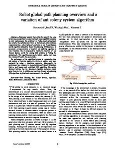
then consists of a sequence of cells and points at which the transition from one cell to another occurs. Planners based on these techniques tend to be more of theoretical interest as they are complex to implement and are inefficient. The path planner implemented in this work is much influenced by the Distance Transform Method [7]. Unlike most path planner, the method considers the task of path planning to find paths from the goal location back to the start location. The path planner propagates a distance wave front through all free space grid cells in the environment from the goal cell, as shown in Figure 1. For any starting point within the environment representing the initial position of the mobile robot, the shortest path to the goal is traced by walking down hill via the steepest descent path. The detailed algorithm is described later in this paper.

obstacle

6

5

4

3

2

1

6

5

4

3

2

1

8

7

6

5

1 3 obstacle

8

7

6

6

6

8

7

6

5

9

7

6

5

6

1

4

1

1

goal 1

1

1

1

2

2

2

3

3

3

4

4

4

Fig. 1. Distance Transform Path Planning

The above three common methods are consider global path planner, which require environment to be known before hand to a certain extend. A local navigation need no a prior knowledge of the environment. One very popular local navigation method is the Potential Field [8] technique. The metaphor suggested by potential field is that the robot be represented as a point in configuration space is a particle moving under the influence of an artificial potential produced by the goal configuration and obstacle configuration. The resulting gradient of the total potential is treated as an artificial force applied on the robot. At every configuration, the direction of this force which is used to guide the robot is considered the most promising direction of motion (collision-free). The other local navigation is the Dynamic Windows Approach [9], [10]. The method takes into account the dynamic and the kinematic constraints of the robot. Addition to these constraints, the obstacles are also taken into account in deciding the admissible velocities to be considered. Among these admissible velocities, a velocity is chosen that maximizes the alignment of the robot with the target and the length of the trajectory. In comparison to global path planner, the local navigation methods can be very effective in dynamic environment. However, they have a major drawback. Since they are essentially fastest decent optimization methods, they can get trapped in local minima. Most of the problem mentioned in the above techniques (global and local) can be resolved by combining the path planner with the local navigation. Distance Transform and Potential Field had been chosen as the two combining components. The reasons for the choice is the ease of integration and implementation, with-

out compromising the navigating robustness of the robot. The following sections will discuss the technique in more detail, including the local navigation, the global path planner and the hybrid. The choice of the two combining methods are also strengthened in the following discussion. The technique is implemented on a Nomad XR4000 mobile robot. III. Local Navigation - Potential Field Method As mentioned in the above section, the robot is imagined as a particle represented by a point in configuration space q. The robot moves under the influence of an artificial field of forces produced by a goal and the obstacles around it. This force on the robot is specified as the negative gradient of a potential function [8]. Expressed as F (q) = −∇V (q)

(1)

where V (q) is the non-negative scalar function over the configuration space of the robot. The V can be considered as specifying the potential energy of the robot at a configuration q. One key property of this potential function is that they are additive, and can be developed independently. The sum of these potentials are usually used to control the robot to move in a desired trajectory, so as to achieve the goal configuration and at the same time avoid obstacles. Hence, an attractive potential can be developed to move the robot towards the goal, and alternatively a repulsive potentials can be developed to avoid collision with the obstacles. Summing these potentials provides a goal-seeking collision-avoiding behaviour. Followings are the formulation for the potential functions and the forces exerting on the robot. The attractive potential can be simply expressed as Vattract (q) =

1 Kattract (q − qdesired )2 2

(2)

thus, the attractive force will be Fattract (q) = Kattract (q − qdesired )

(3)

Kattract is the attraction factor of the function, and q is the current robot configuration, while qdesired is the goal configuration. The effect of the repulsive potential on the robot is obviously opposite from that of the attractive potential. Here we want the obstacles to apply repulsive forces on the robot, where by the magnitude of these forces are inversely proportional to the distance between the robot and the obstacles. On the other hand, repulsive forces from obstacles that are too far away from the robot to post significant danger are undesirable. Therefore, a maximum effective distance of the obstacle from the robot is necessary. Any obstacle further than this effective distance will have no influence on the robot. Thus, the repulsive potential can be expressed as ( 1 Krepul ( d1 − d10 )2 if d < d0 (4) Vrepul (q) = 2 0 if d ≥ d0

and the repulsive force will be ( −Krepul ( d1 − Frepul (q) = 0

1 1 d0 ) d2

if d < d0 if d ≥ d0

(5)

Krepul is the repulsive factor of the function, and d is the distance of the obstacle from the robot, while d0 is the maximum effective distance. The resulting force will therefore be the sum of the attractive force and the repulsive force: Fresult (q) = Fattract (q) + Frepul (q)

(6)

The major drawback of the Potential Field method, is that there is a tendency the robot might get trapped in local minima. This happen when the forces associated with the potentials sum to zero and consequently the robot does not move. This happens when the attractive force towards the goal and the repulsive force are equal and opposite. As a result, the robot will not move. In practice, when the robot is trapped within a local minimum, it does not stop moving. The robot will oscillate around the vicinity of the local minimum. This is due to the imperfect sensory information, thus varying potential forces. This issue is unavoidable especially when the robot is required to move from one room to another in an office-like environment. Most researchers implement recovery methods to solve the local minima problem [11], [12], [13]. Unfortunately, these recovery or avoidance methods do not produce optimized path to the goal configuration. Certain form of searching and redundant movement is required [11], [12]. In addition, heuristics are also needed to detect that the robot is in a local minima situation. IV. Global Path Planner - Distance Transform Distance Transform method [7] proved to be one of the simplest and yet effective way of path planning based on known environment. It is also possible to implement the Distance Transform method in an initially unknown environment. To do this, the robot will have to build the the local map on the move, and at the same time constantly recompute the distance map and the path based on locally available information. This is found to be computationally expensive, and the robot will need to move at a relatively slow speed to accommodate for the mapbuilding and the Distance Transform computation. Therefore, in this paper we will only focus on the method that deal with known environment. Distance Transform method make used of an occupancy grid-based map of the workspace to compute its distance map. Values are assigned to the goal cell and obstacle cells in the initialization stage. Each cell throughout the free configuration space are labelled a value that represents its distance to the goal. These distance values propagation flows around the obstacles. An algorithm that requires iteration until the values in the cells are stabilized, assigns distance values to the rest of the cells. This is done by going through all the cells and apply the algorithm in a fashion similar to raster scanning.

The essential aspect of this approach are that the obstacle cells are set to have very high values (ideally infinity) and are passed over in the raster scan, and the forward then reverse raster scans are repeated until no further changes occur. Any shape of free configuration space can be dealt with in this manner. The resulting Distance Transform is independent of any start point and represent a distance potential field with no local minima [7]. A globally minimal distance path from any start point in free space can be found by a simple steepest decent to the goal cell. The obstacle can be grown by the maximum effective radius of the robot to allow the physical extent of the robot radius and convert the path planning task into a point path problem. An example of obstacle growing by a two cell effective radius is given in Figure 2. Following is the detailed Distance Transform path planning algorithm.

Fig. 2. The black cells represent the actual obstacle cells, while the grey cells are the growth of the obstacles to allow the physical extent of the robot

A. Distance Transform algorithm Let ‘cell’ be a two dimensional array of elements cell [x,y] indexed by x = 0 to xMax+1 and y = 0 to yMax+1, whose elements are to contain the values of the Distance Transform (also referred to as distance values). The edges x = 0, xMax+1 and y = 0, yMax+1 are assumed to contain obstacles (i.e. there is an enclosing wall containing a xMax by yMax cell space). First, we have to initialize all the cells in the array. Let the goal cell contains the minimum distance value (usually zero), the obstacle cells contain the highest possible value representable on the computer (infinity), and the rest of the free space cells contain large values (product of xMax and yMax is a safe value to use). After initializing all the cells, we will compute the distance values for all the free space cell. Occupied and goal cells are unchanged. Other cells are assigned the minimum value of the four vertically and horizontally adjacent neighbours plus one and the four diagonal neighbours √plus two. The diagonal neighbours could be considered a 2 time more than the adjacent neighbours, but for simplistic, it is fine to just make the diagonal neighbour twice as much. The Distance Transform will also work the same way even if the distance values increment for consecutive cells is larger than one. For example letting the increment for consecutive adjacent neighbours be 3 and the diagonal neighbours be 4 will

be:

cell[x,y]idt = min(cell[x+1,y]+3,cell[x+1,y+1]+4, cell[x,y+1]+3,cell[x-1,y+1]+4,cell[x,y]) Once the Distance Transform has been computed, the paths from the start points in the environment can be traced to their goal point. From the start point, we simply walk ‘downhill’, with descending order of the cell’s distance values, until the goal cell is reached. Using the previous example environment in Figure 2, an example of the Distance Transform and the steepest descent path planning is shown in Figure 3 Start cell

will still influence the robot’s movement, hence producing an optimize and adaptable manoeuvre. Succeeding paragraphs discuss the method in more detail. First, using Distance Transform method discussed in Section IV an optimized path is planned from the starting robot position to the goal position. Next, centering on the robot current position, a circle with an empirical radius (say 2 to 4 meters are usually appropriate, depending on the spaciousness of the environment) is created. The intersection of the circumference of the circle and the planned path will be the dynamic sub-goal of the robot. The robot will attempt to reach the sub-goal using the Potential Field method. The use of a circle make the computation of Path Transform not needed. Figure 4 illustrates the method to identify the dynamic sub-goal.

Sub-goal

Start

End

Goal cell

Fig. 3. Distance Transform and steepest descent path planning

There are many global path planner that guaranteed to reach the target for a mobile robot working in a 2dimensional workspace. Several issues were taken into consideration when deciding on a path planner to be implemented in this work. Besides the ease of implementation, another main concern is the potential to extent the planner to work in a dynamic environment. Most global path planner like Roadmap and Cell Decomposition perform a search through a particular graph or map to plan a path from the start configuration to the target configuration. That means the above methods can only execute the planning task with the knowledge of the start and goal configuration. On the other hand, Distance Transform only generate the distance map once based on the goal configuration (without knowledge of the start point). The robot can start from any free space location in the map. This allows the robot to be “disturbed” while it is pursuing the path towards the goal based on steepest decent method. Unlike the other global path planner, which have to replanned the path when the robot is removed from its original planned path. Hence the Distance Transform method provide an avenue to enhance the static path planner to one that is more dynamic and adaptive. V. Having the Best of Both Worlds In this proposed method, we assumed that we have information of the general layout of the environment. The information may be incomplete or inaccurate to certain extent. Using the available environment information, a grid map is generated. The fundamental concept of this technique is to generate an initial path to the goal configuration based on the available grid map, a dynamic goal set along the planned path will then guide the robot to its final desired configuration. The robot’s movement is not restricted just on the planned path. Unknown and/or moving obstacles

(a) Robot at starting position

Robot current position

Sub-goal

(b) Robot moving Fig. 4. Identifying the sub-goal. Note that in (b), the intercept with a lower Distance Value is chosen.

In the case when there are two intersections along the planned path, the cell with the lower Distance Value is used. This ensures that the sub-goal will always progress towards the main goal position. On the other hand, if no intersections is found, the robot is most probably at a location where the planned path is out of range of the radius of that circle. In this situation, the radius of the circle is increased until an intersections with the planned path is found. The above method reduces the level of commitment inherent in a planned path. The reactive control of Potential Field method adapts the motion of the robot in response to information obtained during execution while still following the “local-minima-free” preplanned path.

VI. Implementation and Results The navigation of Nomad XR4000 mobile robot is implemented in a laboratory environment. The workspace contains possible local minima (i.e. concave obstacles), and at certain instances required the robot to manoeuvre through narrow door passage. Figure 5 shows a simple implementation of the robot moving from one location A to room B. The straight and defined line represents the preplanned path using the Distance Transform method, while the slightly staggered line represents the actual path under the influence of Potential Function. The preplanned path served only as a guide for the mobile robot. In situation where no unknown obstacle is in the path, the robot will try to maintain a path that is very close to the preplanned one. Note that the path is slightly more wavy near and at the door passage, as repulsive forces are more intense at that region.

Goal

(a) Robot trapped in a local minima (Starting from B)

Possible local minima

Preplanned path using Distance Transform

(b) Navigation through door passage, avoiding Local Minima (Starting from B and goal at A) Actual path of robot using the Hybrid method

Fig. 6. Solving the local minima problem

Preplanned path

Fig. 5. Navigation from Location A to Room B

Figure 6 shows the efficacy of our Hybrid Method. Figure 6a shows the robot trapped in local minima while starting from location B and trying to achieve the goal. On the other hand, Figure 6b demonstrates the robot negotiating through the door passage and avoiding the possible local minima while moving from room B to location A. In Figure 6a, only Potential Field method is used to navigate to the goal configuration, whereas in Figure 6b, the combined global and local navigation method discussed in Section V was implemented. The navigation implementation shown in Figure 7 is a continuation from Figure 6b. The planned path is deliberately generated to be close to the wall along the corridor. Noticed that the actual robot movement is able to maintain a safe distance away from the wall to avoid the risk of collision with the wall. This is due to the fact that the robot is still influenced by the repulsive force exerted by the wall during execution. The loose coupling between the Potential Field method and the preplanned path allows the robot to react more flexibly to unknown obstacles. The robot will also avoid moving obstacles in the same way. It can be seen from the above implementations that the Potential Field method which is effective for real-time obstacle avoidance is able to integrate satisfactorily into the global path planner which on the other hand promises a “local minima free” path.

Actual path

Fig. 7. Navigation from Room B to Location A

VII. Conclusion This paper described a simple yet effective algorithm in mobile robot navigation in an indoor environment. The algorithm make used of two existing techniques, Distance Transform and Potential Field, to produce a hybrid of a global path planner and a reactive navigation method. The proposed technique solved the shortcoming in the inefficiency of reactive navigation, and avoided the problem of local minima. In addition, the hybrid encompasses the strength of having an optimized planned path, and yet retaining the advantages of a dynamic reactive control. References [1]

J.S.B, Planning Shortest Paths, Ph.D. thesis, Dept. of Operations Research, Stanford University, 1986.

[2] [3] [4]

[5]

[6] [7]

[8] [9] [10]

[11] [12]

[13]

V. Akman, Unobstructed Shortest Paths in Polyhedral Environments, Lecture Notes in Computer Science. Springer-Verlag, 1987. C. ’Dnliang and C.K. Yap, “Retraction: A new approach to motion planning,” Proceeding of the 15th ACM Symposium on the Theory of Computing, Boston, pp. 207–220, 1983. C. Mirolo and E. Pagello, “A cell decomposition approach to motion planning based on collision detection,” Proceedings of the Int. Conf. on Advanced Robotics (ICAR’95), pp. 481–488, 1995. Nora H. Sleumer and Nadine Tschichold-Grman, “Exact cell decomposition of arrangements used for path planning in robotics,” Tech. Rep., Institute of Theoretical Computer Science Swiss Federal Institute of Technology Zurich, Switzerland, 1999. B. Chazelle, “Approximation and decomposition of shapes,” in Aspects of Robotics, Lawrence Elbraum, J.T. Schwartz and C.K. Yap, Eds., vol. 1 of Advances in Robotics. 1987. Ray Jarvis, “Distance transform based path planning for robot navigation,” in Recent trends in mobile robots, Yuan F. Zheng, Ed., vol. 11 of Robotics and Intelligent Systems, chapter 1. World Scientific, 1993. Oussama Khatib, “Real-time obstacle avoidance for manipulators and mobile robots,” International Journal of Robotics Research, vol. 5, no. 1, pp. 90–98, 1986. D. Fox, W. Burgard, and S. Thurn, “The dynamic window approach to collision avoidance,” IEEE Transactions on Robotics and Automation, 1997. Oliver Brock and Oussama Khatib, “High-speed navigation using the global dynamic window approach,” Proceedings of the International Conference on Robotics and Automation, vol. 1, pp. 341–346, 1999. Chengqing Liu, “Sensor based local path planning for mobile robot,” M.S. thesis, National University of Singapore, 2000. Chengqing Liu, Marcelo H. Ang Jr., and H. Krishnan, “Virtual obstacle concept for local minimum recovery in potential field based navigation,” Proceedings of the 2000 IEEE International Conference on Robotics and Automation, San Francisco, USA, pp. 983–988, April 2000. V. Lumelsky and A.A.Stepanov, “Path planning strategies of a point mobile automation moving amidst unknown obstacles of arbitrary shape,” Algorithmica, vol. 2, pp. 403–430, 1987.