GLMP- Realtime Pedestrian Path Prediction using Global and Local Movement Patterns Aniket Bera, Sujeong Kim, Tanmay Randhavane, Srihari Pratapa and Dinesh Manocha http://gamma.cs.unc.edu/RCrowdT/GLMP/ Abstract— We present a novel real-time algorithm to predict the path of pedestrians in cluttered environments. Our approach makes no assumption about pedestrian motion or crowd density, and is useful for short-term as well as long-term prediction. We interactively learn the characteristics of pedestrian motion and movement patterns from 2D trajectories using Bayesian inference. These include local movement patterns corresponding to the current and preferred velocities and global characteristics such as entry points and movement features. Our approach involves no precomputation and we demonstrate the real-time performance of our prediction algorithm on sparse and noisy trajectory data extracted from dense indoor and outdoor crowd videos. The combination of local and global movement patterns can improve the accuracy of long-term prediction by 12-18% over prior methods in high-density videos.
I. I NTRODUCTION The problems of video-based pedestrian detection and path prediction have received considerable attention in robotics, intelligent vehicles, and video surveillance. As mobile robots are increasingly used for service tasks, it is important for these robots to perceive the intent and trajectory of humans for collaborative collision avoidance. In the context of (semi)autonomous driving, it is important to compute precise estimates of the current and future positions of each pedestrian with respect to the moving vehicle for collision-free navigation. In computer vision and multimedia applications, pedestrian movement detection and prediction is used for detecting abnormal activities or behaviors. Pedestrian path prediction from videos or other sensor data is regarded as a challenging problem. In general, pedestrians have varying behaviors and can change their speed to avoid collisions with the obstacles in the scene and other pedestrians. In high density or crowded scenarios, the pairwise interactions between the pedestrians tend to increase significantly. As a result, the highly dynamic nature of pedestrian movement makes it hard to estimate their current or future positions. Furthermore, many applications need real-time prediction capabilities to estimate the positions of large number of pedestrians in a short time. Some of the commonly used algorithms for predicting the path of pedestrians are based on tracking filters. These include Kalman filter, particle filter, and their variants. Other approaches are based on hidden Markov models. Many of these trackers also use motion models for pedestrian movement to improve the prediction accuracy. The simplest All the authors from the Department of Computer Science, University of North Carolina at Chapel Hill, USA
[email protected]
Fig. 1: Improved Prediction We demonstrate the improved accuracy of our pedestrian path prediction algorithm (GLMP) over prior real-time prediction algorithms (BRVO, Const Vel, Const Accel) and compare them with the ground truth. We observe upto 18% improvement in accuracy. motion models are based on constant velocity or constant acceleration assumptions [7]. Other algorithms are based on sophisticated motion models based on social forces [12], reciprocal velocity obstacles [28], dynamic social behaviors [24], etc. to model pairwise interactions between the pedestrians, or combine Bayesian statistical inference with velocityspace reasoning [14] for computing individualized motion model for each pedestrian. In practice, all these methods only capture local interactions and movements, which are mostly useful for short-term deviations from goal-directed paths. However, they may not work well in dense situations where the pedestrians make frequent stops or long-term predictions.
Main Results: In this paper, we present a novel algorithm to learn pedestrian local and global movement patterns from sparse 2D pedestrian trajectory data using Bayesian Inference. Our approach is general, makes no assumption about pedestrian movement or density, and performs no precomputation. We use the trajectory data information over a sequence of frames to predict the future pedestrian states using Ensemble Kalman Filters (EnKF) and Expectation Maximization (EM). The state information is used to compute movement-flow information of individual pedestrians and coherent pedestrian clusters using a mixture of motion models. The global movement features are combined with local motion patterns computed using Bayesian reciprocal velocity obstacles to compute the predicted state of each pedestrian. The combination of Global and Local Movement Patterns (i.e. GLMP) corresponds to computing dynamically
Fig. 2: We highlight various components of our real pedestrian path prediction algorithm. Our approach computes both local and global movement patterns using Bayesian inference from 2D trajectory data and combines them to improve prediction accuracy. varying individualized motion model for each pedestrian. Overall, our approach offers the following benefits: •
• •
Our algorithm is general and can compute global and local movement patterns in real-time with no prior learning. We can robustly handle sparse and noisy trajectory data generated using current online pedestrian trackers. We observe upto 18% increase in prediction accuracy as compared to prior real-time methods that are based on simple filters or only local movement patterns.
We highlight the performance of GLMP to predict the positions of pedestrians using trajectory data extracted from a variety of video datasets consisting of 30-400 pedestrians. Our approach can predict the positions of tens of pedestrians in around 40-50 milliseconds over long-intervals. Furthermore, we demonstrate its benefits over prior real-time prediction algorithms. The rest of our paper is organized as follows. Section II gives a brief overview of prior work in pedestrian path prediction, tracking, and motion models. We present our movement flow learning algorithm in Section III and use that for path prediction. We highlight its performance on different crowd video datasets in Section IV and compare its performance with prior methods. II. R ELATED W ORK In this section, we give a brief overview of prior work on motion models and pedestrian path prediction. A. Pedestrian-Tracking with Motion Models Prior work in pedestrian tracking [6], [15] attempts to improve tracking accuracy by making simple assumptions about pedestrian movement, such as constant velocity and constant acceleration. In recent years, long-term motion models and pairwise interaction rules have been combined with tracking
to improve the accuracy. Liao et al. [18] extract a Voronoi graph from the environment and predict people’s motion along the edges. Many techniques have been proposed for short-term prediction using motion models. Luber et al. [19] apply Helbing’s social force model to track people using a Kalman-filter based tracker. Mehran et al. [21] also apply the social force model to detect people’s abnormal behaviors from video. Pellegrini et al. [24] use an energy function to build up a goal-directed short-term collision-avoidance motion model. Bera et al. [4], [5], [2] use reciprocal velocity obstacles and hybrid motion models to improve the accuracy of pedestrian tracking. B. Path Prediction and Robot Navigation Robots navigating in complex, noisy, dynamic environments have prompted the development of other forms of trajectory prediction. Fulgenzi et al. [10] use a probabilistic velocityobstacle approach combined with the dynamic occupancy grid; this method assumes constant linear velocity motion of the obstacles. DuToit et al. [8] present a robot planning framework that takes into account pedestrians’ anticipated future location information to reduce the uncertainty of the predicted belief states. Other techniques use potential-based approaches for robot path planning in dynamic environments [25]. Some methods learn the trajectories from collected data. Ziebart et al. [30] use pedestrian trajectories collected in the environment for prediction using Hidden Markov Models. Bennewitz et al. [1] apply Expectation Maximization clustering to learn typical motion patterns from pedestrian trajectories, before using Hidden Markov Models to predict future pedestrian motion. Henry et al. [13] use reinforced learning from example traces, estimating pedestrian density and flow with a Gaussian process. Kretzschmar et al. [16] consider pedestrian trajectories as a mixture probability distribution of a discrete as well as a continuous distribution and then use Hamiltonian Markov chain Monte Carlo sampling for prediction. Kuderer et al. [17] use maximum entropy based learning to learn pedestrian trajectories and use a hierarchical
optimization scheme to predict future trajectories. Many of these methods involve a priori learning, and may not work in new or unknown environments. Trautman et al. [27] have developed a probabilistic predictive model of cooperative collision avoidance and goal-oriented behavior for robot navigation in dense crowds. Guzzi et al. [11] present a distributed method for multi-robot human like local navigation. Variations of the Bayesian filters for pedestrian path prediction have been studied in [26], [22]. Some of these methods are not suitable for real-time applications or may not work well for dense crowds. III. R EAL - TIME P EDESTRIAN PATH P REDICTION In this section, we present our real-time algorithm that learns movement flows from real-world pedestrian 2D trajectories that are extracted from video. Our approach involves no precomputation or learning, and can be combined with real-time pedestrian trackers. Fig. 2 gives an overview of our approach, including computation of movement flows and using them for pedestrian prediction. The input to our method consists of a live or streaming crowd video. We extract the initial set of trajectories using an online particle-filter based pedestrian tracker. These trajectories are time-series observations of the positions of each pedestrian in the crowd. The various components used in our algorithm are shown in the figure and explained below. The output is the predicted state of each agent that is based on learning the local and global pedestrian motion patterns. A. Pedestrian State Estimation We first define specific terminology used in the paper. We use the term pedestrian to refer to independent individuals or agents in a crowd. We use the notion of state to specify the trajectory characteristics of each pedestrian. We assume that the output of the tracker corresponds to discrete 2D positions. Therefore, our state vector, represented using the symbol x ∈ R6 , consists of components that describe the pedestrian’s movements on a 2D plane: x = [p vc vpref ]T ,
(1)
c
where p is the pedestrian’s position, v is its current velocity, and vpref is the preferred velocity on a 2D plane. The preferred velocity corresponds to the predicted velocity that a pedestrian would take to achieve its intermediate goal if there were no other pedestrians or obstacles in the scene. We use the symbol S to denote the current state of the environment, which corresponds to the state of all other pedestrians and the current position of the obstacles in the scene. The state of the crowd, which consists of individual pedestrians, is a S union of the set of each pedestrian’s state X = i xi , where subscript i denotes the ith pedestrian. The trajectories extracted from a real-world video tend to be noisy and may have incomplete tracks [9]; thus, we use
Fig. 4: Global vs Local Movement Patterns The blue trajectories indicate prior tracked data. The red dots indicate local predicted patterns retrieved from learning macro and microscopic simulation models, The shaded (green-blue) path represent the global movement patterns learned from the path data in that cluster Bayesian-inference technique to compensate for any errors and to compute the state of each pedestrian [14]. At each time step, the observation of a pedestrian computed by a tracking algorithm corresponds to the position of each pedestrian on the 2D plane, denoted as zt ∈ R2 . The observation function h() provides zt of each pedestrian’s true state x ˆt with sensor 2 error r ∈ R , which is assumed to follow a zero-mean Gaussian distribution with covariance Σr : z t = h(ˆ xt ) + r, r ∼ N (0, Σr ).
(2)
h() is the tracking sensor output. We use the notion of a state-transition model f () which is an approximation of true real-world pedestrian dynamics with prediction error q ∈ R6 , which is represented as a zero-mean Gaussian distribution with covariance Σq : xt+1 = f (xt ) + q, q ∼ N (0, Σq ).
(3)
We can use any local navigation algorithm or motion model for function f (), which computes the local collision-free paths for the pedestrians in the scene. More details are given below. Our algorithm uses an Ensemble Kalman Filter (EnKF) and Expectation Maximization (EM) with the observation model h() and the state transition model f () to estimate the most likely state x of each pedestrian [14]. In particular, EnKF predicts the next state based on the transition model and the covariance matrix Σq and updates them whenever a new observation is available. The EM step computes Σq to maximize the likelihood of the state estimation. Pedestrian Clusters Our approach is targeted towards computing the movement flows of pedestrians in dense settings. It is not uncommon for some nearby pedestrians to have similar flows. As a result, we compute clusters of pedestrians in a crowd based their positions, velocity, inter-pedestrian distance, orientations, etc. In particular, we use a bottom-up hierarchical clustering approach, as they tend to work better for small clusters. Initially, we assign each pedestrian to a
Fig. 3: Prediction Outputs We test our approach on a variety of crowd datasets with varying density. Our approach had a benefit of upto 18% better prediction at a 5 second time horizon for some high-density datasets. Yellow lines represent past tracked trajectories whereas the red dots represent predicted motion.
separate cluster that consists of a single pedestrian. Next, we merge these clusters based on computing the distance between various features highlighted above. Our approach is based on group-expand procedure [20] and we include many pedestrian movement related features to compute the clusters. We compute a connectivity graph among the pedestrians and measure the graph density based on intra-cluster proximity [5]. Eventually, we use a macroscopic model to estimate the movement of each cluster and use this model to predict their global movement. B. Global Movement Pattern A key aspect of our approach is to compute global movement patterns that can be used to predict the state of each pedestrian. These movement patterns describe the trajectorylevel motion or behavior at a certain position at time frame t. The patterns include the movement of the pedestrian during the past w frames, which we call time window, and the intended direction of the movement (preferred velocity) at this position. In our formulation, we represent each movement feature vector as a six-dimensional vector: b = [p vavg vpref ]T ,
(4)
where p, vavg , and vpref are each two-dimensional vectors representing the current position, average velocity during past w frames, and estimated preferred velocity computed as part of state estimation, respectively. vavg can be computed from (pt − pt−w )/w ∗ dt, where dt is the time step. We use the notion of average velocity over the last w frames as that provides a better estimate of pedestrian movement. In a dense setting, some pedestrians may suddenly stop or change their local directions as they interact with other pedestrians. As a result, the duration of the time window, w, is set based on the characteristics of a scene. If we use small time windows, the movement flows will be able to capture the details in dynamically changing scenes. On the other hand, larger time windows tend to smooth out abrupt changes in pedestrian motion and are more suitable for scenes that have little change in pedestrians’ movement.
At every w steps, we compute the new trajectory features for each pedestrian in the scene, using Equation 4. Moreover, we group the similar features and find K most common trajectory patterns, which we call global movement patterns. We use recently observed behavior features to learn the timevarying movement flow. This set of K global movement patterns B = {B1 , B2 , ..., BK } is computed as follows: argmin B
K X X
dist(bi , µk ),
(5)
k=1 bi ∈Bk
where bi is a movement feature vector, µk is a centroid of each flow movement pattern, and dist(bi , µk ) is a distance measure between the arguments. In our case, the distance between two feature vectors is computed as dist(bi , bj ) = c1 kpi − pj k
+ c2 (pi − viavg w dt) − (pj − vjavg w dt)
+ c3 (pi + vipref w dt) − (pj − vjpref w dt) ,
(6)
which corresponds to the weighted sum of the distance among three points: current positions, previous positions and estimated future positions that are extrapolated using v pref , c1 , c2 , and c3 as the weight values. Comparing the distance between the positions rather than mixing the points and the vectors eliminates the need to normalize or standardize the data. We use the movement feature of the cluster to compute the predicted state at time t, Sgt . C. Local Movement Pattern During each frame, some of the pedestrians are modeled as discrete agents, while the clusters are treated using macroscopic techniques. Based on the observations and state information, we estimate the motion model for these discrete agents and pedestrian clusters. For each individual pedestrian represented as a discrete agent, we compute the motion model that best fits its position as tracked over recent frames i.e. we compute the features per-agent and predict motion patterns locally. We choose the “best” local motion model from a fixed set of choices. The common choices are based on social forces, reciprocal velocity obstacles or Boids. In our case, the “best” motion model is the one that most accurately matches the immediate past states based on a given error
metric. This “best” motion model is computed using a local optimization algorithm [3], which automatically finds the motion model parameters that minimize that error metric. A motion model (microscopic or macroscopic) is defined as an algorithm f (defined in Equation 3) that starts with a collection of agent states Xt , and computes the new states Xt+1 for these agents. It represents their motion over a timestep towards the agents’ immediate goals G: Xt+1 = f (Xt , G, P),
(7)
where P denotes the individual pedestrian parameters. Formally, at any timestep t, we define the agents’ (k+1)-states (as computed by the tracker and state estimation) St−k:t : St−k:t =
t [
Si .
(8)
Fig. 5: Improved Prediction We demonstrate the improved accuracy of our pedestrian path prediction algorithm (GLMP) over prior real-time prediction algorithms (BRVO, Const Vel, Const Accel).
i=t−k
IV. A NALYSIS Similarly, the motion model corresponding to computed agents’ state f (St−k:t , P) can be defined as: f (St−k:t , P) =
t [
f (Xi , G, P),
(9)
i=t−k
initialized with Xt−k = St−k and G = St . At timestep t, considering the agents’ k-states St−k:t , computed states f (St−k:t , P) and a user-defined error metric error(), our algorithm computes: = argmin error(f (St−k:t , P), St−k:t ), Popt,f t
(10)
P
where Popt,f is the parameter set which, at timestep t, results t in the closest match between the states computed by the motion algorithm f and the agents’ k-states. D. Prediction Output For every pedestrian, we compute both the global and local movement patterns separately. In practice, we observed that for lower density scenarios, local movement patterns are more useful than global patterns and vice-versa. Our final predicted state is a weighted average of the individual predicted states generate from the local and global patterns as: g l Sp t = (1 − w) ∗ St + w ∗ St ,
(11)
l where Sp t is the final predicted state at time t, St is the state predicted from the local patterns and the Sgt is the state predicted from global patterns or from the movement flows. As a general rule of thumb, w varies from 0 to 1 and is computed based on the pedestrian density. We use a larger weight for higher density. In order to perform longterm predictions (5-6 seconds or even longer), we tend to increase w as the global movement patterns provide better estimates for pedestrian position.
In this section, we highlight the prediction results using GLMP algorithm and compare its performance with prior method. We have applied it to the 2D trajectories generated from different crowd videos and compared the prediction accuracy with the ground truth data, that was also generated using a pedestrian tracker. The underlying crowd videos have different pedestrian density corresponding to low (i.e. less than 1 pedestrian per squared meter), medium (12 pedestrians per squared meter), and high (more than 2 pedestrians per squared meter). We highlight the datasets, their crowd characteristics, and the prediction accuracy of different real-time algorithms for short-term and long-term prediction in Table 1. We also analyze the accuracy of our appraoch based on varying the pedestrian density (Fig. 7) and the frame sampling rate (Fig. 8). The performance of the method with noisy data (i.e sensor noise) is also analyzed. Finally, we perform a qualitative and quantitative comparison to other real-time pedestrian path prediction algorithms. We include comparisons to constant velocity (ConstVelocity) and constant acceleration (ConstAccel) motion models, which are widely used for pedestrian tracking and prediction in robotics and computer vision [7]. We also compare the accuracy with recent methods that use more sophisticated motion models (LTA and ATTR) to compute local movement patterns [24], [29]. Finally, we also compare the accuracy with the Bayesian reciprocal velocity obstacle (BRVO) algorithm [14] that computes a more individualized motion model for estimating local movement patterns. A. Noisy Data Sensor noise is an important concern in pedestrian prediction algorithms. In order to evaluate the impact of noise, we add synthetic noise to the datasets and compare the performance of GLMP vs. other algorithms on these benchmarks: IITF [4], ETH and Campus [23] datasets.
Dataset
Challenges
Density
# Tracked
NDLS-1 IITF-1 IITF-3 IITF-5 NPLC-1 NPLC-3 Students Campus seq hotel Street
BV, PO, IC BV, PO, IC, CO BV, PO, IC, CO BV, PO, IC, CO BV, PO, IC BV, PO, IC, CO BV, IC, PO BV, IC, PO IC, PO IC, PO
High High High High Medium Medium Medium Medium Low Low
131 167 189 71 79 144 65 78 390 34
ConstVelocity 1 sec 5 secs 55.3% 32.0% 63.5% 33.4% 61.1% 29.1% 59.2% 28.8% 76.1% 63.9% 77.9% 70.1% 65.0% 58.2% 62.4% 57.1% 74.7% 67.8% 78.1% 70.9%
Kalman 1 sec 53.1% 63.9% 63.6% 61.7% 78.2% 79.1% 66.9% 63.5% 76.7% 78.9%
Filter 5 secs 37.9% 39.1% 31.0% 29.1% 65.8% 71.9% 61.0% 59.0% 68.3% 71.0%
BRVO 1 sec 5 secs 56.5% 42.0% 65.3% 41.8% 67.6% 37.5% 62.9% 30.1% 79.9% 69.0% 80.8% 74.4% 69.1% 63.6% 66.4% 59.1% 76.9% 69.2% 81.4% 71.2%
GLMP 1 sec 5 secs 60.2% 51.2% 71.2% 50.5% 68.4% 45.7% 64.6% 40.0% 82.3% 72.5% 84.3% 78.1% 72.2% 66.8% 69.6% 59.5% 79.5% 70.1% 83.8% 72.7%
TABLE I: Crowd Scene Benchmarks: We highlight many attributes of these crowd videos, including density and the number of tracked pedestrians. We use the following abbreviations about some characteristics of the underlying scene: Background Variations (BV), Partial Occlusion (PO), Complete Occlusion (CO) and Illumination Changes (IC). We highlight the results for short-term prediction (1 sec) and long term prediction (5 sec). We notice that our GLMP algorithm results in higher accuracy for long-term prediction and dense scenarios. More details are given in Section IV(B).
Fig. 6 compares the prediction accuracy of GLMP, constant velocity, constant acceleration and BRVO, by comparing the predicted positions to the actual ground truth data extracted using pedestrian trackers. We use these noise levels, 0.05m, 0.1m, and 0.15m to simulate different sensor variations. During the prediction step, we assume that no further information is given when we are predicting the future state, and our best guess is that the pedestrians move according to their preferred velocity computed using the movement patterns. For GLMP, the pedestrian’s movement direction changes when there is any interaction with obstacles or other pedestrians as observed based on local and global movement patterns. Fig. 7 shows the fraction of correctly predicted paths within varying accuracy thresholds. At an accuracy threshold of 0.5m, GLMP has higher accuracy than BRVO and offers considerable benefits over constant velocity, constant acceleration models even with little noise. As the noise increases, the benefit in prediction accuracy using GLMP also increases.
C. Varying the Pedestrian Density We use a variation of crowd videos with different densities (Low, Medium and High) and compare GLMP’s error to that of BRVO, constant velocity and constant acceleration models (see Fig. 7). Both the constant velocity and constant acceleration models have large variations in error for different regions of the scenario with varying densities. In contrast, the GLMP approach performs well across all densities because it can dynamically adapt the parameters for each agent for each frame and learn global as well as local motion patterns. We observe higher accuracy benefits in high density scenarios due to the computation of global movement patterns.
B. Long-term Prediction Accuracy Being able to predict a trajectory over a longer time-horizon is important for service robots and autonomous vehicles. Our approach is able to perform long-term prediction (56 seconds) with much higher accuracy than prior methods (see Table 1). We use a simple prediction metric to evaluate the accuracy of both, long and short term prediction. A prediction is counted as “successful” when the estimated mean error between the prediction result and the ground-truth value at that time instance is less than 0.8 meter in ground space coordinates. The average human stride length is about 0.8 meter and we consider the prediction to be incorrect if the mean error is more than this value. We define prediction accuracy as the ratio of the number of “successful” predictions and total number of tracked pedestrians in the scene. We use our algorithm for long and short term prediction across a large number of datasets, highlighted in Table 1.
Fig. 7: Errors for varying Pedestrian Densities (lower is better). In low-density scenarios, local movement patterns (e.g BRVO) are able to predict the positions well, but are more accurate than const. velocity and const. acceleration. We observe improved accuracy with GLMP, as the pedestrian density increases. D. Varying the Sampling Rate GLMP works very well on data with very low frame-rate, when the video or data is sampled at large intervals. In low FPS videos, there is less temporal direct pixel overlap between frames. In a way, this is also a metric for evaluating the accuracy of our prediction algorithm. In order to evaluate the performance, we evaluated the accuracy on the Street,
Fig. 6: Prediction Accuracy vs. Sensor Error (higher is better) We increase the sensor noise (Gaussian) from left to right and highlight the prediction accuracy across various distance thresholds. The X-axis represents the percentage of correctly predicted paths within varying accuracy thresholds. In this GLMP results in more accurate predictions, as compared to BRVO, Constant Velocity, Constant Acceleration. As the sensor noise increases (c), we observe more significant benefit.
seq hotel, seq eth and IITF datasets at varying frame-rates. Fig. 8 shows the graph of the mean error versus the sampling interval. The graph in the figure shows that our method performs very well compared to BRVO, constant velocity and constant acceleration model across all the sampling rates.
Fig. 8: Error vs Sampling Interval As the sampling interval increases, the error from Constant Velocity, Constant Acceleration and BRVO grows much larger than that from GLMP.
E. Comparison with Prior Methods We directly compare our results with the prediction results of LTA [23] and ATTR [29], which report performance numbers for some of the same benchmarks. Unlike GLMP, both these methods require offline preprocessing or annotation. We also compare GLMP with BRVO along with LTA and ATTR on Street, NDLS, IITF, seq hotel and seq eth datasets, all sampled every 1.5 seconds, and measure mean prediction error for every agent in the scene during the entire video sequence. The metric used was error reduction comparison, and is measured as improvement in percentage of error reduction over the LIN model for different algorithms. The results are shown in Fig. 9. Our method outperforms LTA and ATTR with 24-47% error reduction rate across the three different scenarios. LTA and ATTR use the ground truth destinations
for prediction; LTA+D and ATTR+D use destinations learned offline, as explained in [29]; ATTR+D uses grouping information learned offline. Even though GLMP is an online and real-time method, it shows significant improvement in prediction accuracy on all the datasets, producing less error than other approaches.
Fig. 9: Error Reduction Comparison We compare the improvements of our method, LTA, ATTR and BRVO over LIN (linear velocity) model. Our method (GLMP) outperforms LTA, ATTR with 24-47% error reduction rate in all three different scenarios. V. L IMITATIONS , C ONCLUSIONS , AND F UTURE W ORK We present a novel real-time algorithm for pedestrian path prediction. The main idea is to learn the local and global movement patterns using Bayesian inference. Our approach can handle low as well as high density videos and is useful for short-term and long-term prediction. We have highlighted its performance on many benchmarks and demonstrate the improvements in accuracy over prior real-time algorithms. Our approach has some limitations. The underlying formulation does not model many other aspects of pedestrian behavior, including physiological and psychological pedestrian traits as well as age, gender or external environmental factors. The estimation techniques relies on Bayesian inferences
and that may not work well in some cases. In terms of future work, we would like to overcome these limitations. Furthermore, we would like to evaluate their performance with robots, e.g. service robots or autonomous vehicles, navigating through pedestrians.
[16] Henrik Kretzschmar, Markus Kuderer, and Wolfram Burgard. Learning to predict trajectories of cooperatively navigating agents. In Robotics and Automation (ICRA), 2014 IEEE International Conference on, pages 4015–4020. IEEE, 2014.
VI. ACKNOWLEDGEMENTS
[18] L. Liao, D. Fox, J. Hightower, H. Kautz, and D. Schulz. Voronoi tracking: Location estimation using sparse and noisy sensor data. In Proc. of the 2003 IEEE/RSJ International Conference on Intelligent Robots and Systems (IROS), volume 1, pages 723–728. IEEE, 2003.
This work was supported by NSF awards 1117127, 1305286, ARO contract W911NF-14-1-0437, and a grant from the Boeing company. R EFERENCES [1] M. Bennewitz, W. Burgard, G. Cielniak, and S. Thrun. Learning motion patterns of people for compliant robot motion. The International Journal of Robotics Research, 24(1):31–48, 2005. [2] Aniket Bera, Nico Galoppo, Dillon Sharlet, Adam Lake, and Dinesh Manocha. Adapt: real-time adaptive pedestrian tracking for crowded scenes. In ICRA, 2014. [3] Aniket Bera, Sujeong Kim, and Dinesh Manocha. Efficient trajectory extraction and parameter learning for data-driven crowd simulation. In Graphics Interface, 2015. [4] Aniket Bera and Dinesh Manocha. Realtime multilevel crowd tracking using reciprocal velocity obstacles. In ICPR, 2014. [5] Aniket Bera and Dinesh Manocha. REACH: Realtime crowd tracking using a hybrid motion model. ICRA, 2015. [6] J. Cui, H. Zha, H. Zhao, and R. Shibasaki. Tracking multiple people using laser and vision. In Proc. of the IEEE/RSJ International Conference on Intelligent Robots and Systems (IROS), pages 2116– 2121. IEEE, 2005. [7] Alberto Del Bimbo and Fabrizio Dini. Particle filter-based visual tracking with a first order dynamic model and uncertainty adaptation. Computer Vision and Image Understanding, 2011. [8] N.E. Du Toit and J.W. Burdick. Robotic motion planning in dynamic, cluttered, uncertain environments. In Robotics and Automation (ICRA), 2010 IEEE International Conference on, pages 966–973, 2010. [9] Markus Enzweiler and Dariu M Gavrila. Monocular pedestrian detection: Survey and experiments. IEEE PAMI, 2009. [10] C. Fulgenzi, A. Spalanzani, and C. Laugier. Dynamic obstacle avoidance in uncertain environment combining pvos and occupancy grid. In Robotics and Automation, 2007 IEEE International Conference on, pages 1610–1616, 2007. [11] J. Guzzi, A. Giusti, L.M. Gambardella, G. Theraulaz, and G.A. Di Caro. Human-friendly robot navigation in dynamic environments. In Robotics and Automation (ICRA), 2013 IEEE International Conference on, pages 423–430, May 2013. [12] D. Helbing and P. Molnar. Social force model for pedestrian dynamics. Physical review E, 51(5):4282, 1995. [13] P. Henry, C. Vollmer, B. Ferris, and D. Fox. Learning to navigate through crowded environments. In Robotics and Automation (ICRA), 2010 IEEE International Conference on, pages 981–986, 2010. [14] Sujeong Kim, Stephen J Guy, Wenxi Liu, David Wilkie, Rynson WH Lau, Ming C Lin, and Dinesh Manocha. Brvo: Predicting pedestrian trajectories using velocity-space reasoning. The International Journal of Robotics Research, page 0278364914555543, 2014. [15] L. Kratz and K. Nishino. Tracking pedestrians using local spatiotemporal motion patterns in extremely crowded scenes. Pattern Analysis and Machine Intelligence, IEEE Transactions on, (99):11, 2011.
[17] Markus Kuderer, Henrik Kretzschmar, Christoph Sprunk, and Wolfram Burgard. Feature-based prediction of trajectories for socially compliant navigation. In Robotics: science and systems, 2012.
[19] M. Luber, J.A. Stork, G.D. Tipaldi, and K.O. Arras. People tracking with human motion predictions from social forces. In Proc. of the IEEE International Conference on Robotics and Automation (ICRA), pages 464–469, 2010. [20] Clark McPhail and Ronald T Wohlstein. Using film to analyze pedestrian behavior. Sociological Methods & Research, 10(3):347– 375, 1982. [21] R. Mehran, A. Oyama, and M. Shah. Abnormal crowd behavior detection using social force model. In Proc. of the IEEE Conference on Computer Vision and Pattern Recognition,CVPR, pages 935–942, 2009. [22] Andreas Mogelmose, Mohan M. Trivedi, and Thomas B. Moeslund. Trajectory analysis and prediction for improved pedestrian safety: Integrated framework and evaluations. In Intelligent Vehicles Symposium (IV), 2015 IEEE, pages 330–335, June 2015. [23] S. Pellegrini, A. Ess, K. Schindler, and L. Van Gool. You’ll never walk alone: Modeling social behavior for multi-target tracking. In Proc. of the IEEE 12th International Conference on Computer Vision, page 261268, 2009. [24] Stefano Pellegrini, Andreas Ess, Konrad Schindler, and Luc Van Gool. You’ll never walk alone: Modeling social behavior for multi-target tracking. In ICCV, 2009. [25] N. Pradhan, T. Burg, and S. Birchfield. Robot crowd navigation using predictive position fields in the potential function framework. In American Control Conference (ACC), 2011, pages 4628–4633, 2011. [26] Nicolas Schneider and Dariu M. Gavrila. Pedestrian path prediction with recursive bayesian filters: A comparative study. In Pattern Recognition - 35th German Conference, GCPR 2013, Saarbr¨ucken, Germany, September 3-6, 2013. Proceedings, pages 174–183, 2013. [27] P. Trautman, J. Ma, R.M. Murray, and A. Krause. Robot navigation in dense human crowds: the case for cooperation. In Robotics and Automation (ICRA), 2013 IEEE International Conference on, pages 2153–2160, May 2013. [28] J. Van Den Berg, S. Guy, M. Lin, and D. Manocha. Reciprocal n-body collision avoidance. Robotics Research, page 319, 2011. [29] K. Yamaguchi, A.C. Berg, L.E. Ortiz, and T.L. Berg. Who are you with and where are you going? In Proc. of the 2011 IEEE Conference on Computer Vision and Pattern Recognition (CVPR), pages 1345–1352, june 2011. [30] Brian D. Ziebart, Nathan Ratliff, Garratt Gallagher, Christoph Mertz, Kevin Peterson, J. Andrew Bagnell, Martial Hebert, Anind K. Dey, and Siddhartha Srinivasa. Planning-based prediction for pedestrians. In Proc. of the 2009 IEEE/RSJ international conference on Intelligent robots and systems (IROS), IROS’09, pages 3931–3936, Piscataway, NJ, USA, 2009. IEEE Press. [31] Brian D Ziebart, Nathan Ratliff, Garratt Gallagher, Christoph Mertz, Kevin Peterson, James A Bagnell, Martial Hebert, Anind K Dey, and Siddhartha Srinivasa. Planning-based prediction for pedestrians. In IROS, pages 3931–3936, 2009.