Hybridisations of Variable Neighbourhood and Modified Simplex ...

Proceedings of the International MultiConference of Engineers and Computer Scientists 2010 Vol III, IMECS 2010, March 17 - 19, 2010, Hong Kong

Hybridisations of Variable Neighbourhood and Modified Simplex Methods to Harmony Search Algorithm for Process Optimisations P. Aungkulanon* and P. Luangpaiboon, Member, IAENG Abstract — Nowadays, the engineering problem systems are large and complicated. An effective finite sequence of instructions for solving these problems can be categorised into optimisation and meta-heuristic algorithms. Though the best decision variable levels from some sets of available alternatives cannot be done, meta-heuristics is an alternative for experience-based techniques that rapidly help in problem solving, learning and discovery in the hope of obtaining a more efficient or more robust procedure. All meta-heuristics provide auxiliary procedures in terms of their own tooled box functions. It has been shown that the effectiveness of all meta-heuristics depends almost exclusively on these auxiliary functions. In fact, the auxiliary procedure from one can be implemented into other meta-heuristics. A well-known metaheuristic of harmony search algorithm (HSA) is compared with its hybridisations. HSA is used to produce a near optimal solution under a consideration of the perfect state of harmony of the improvisation process of musicians. This study presents solution procedures via constrained and unconstrained problems with different natures of single and multi peak surfaces including a curved ridge surface. HSA is modified via variable neighbourhood search method (VNSM) philosophy including a modified simplex method (MSM). The basic idea is the change of neighbourhoods during searching for a better solution. The hybridisations proceed by a descent method to a local minimum exploring then, systematically or at random, increasingly distant neighbourhoods of this local solution. The results show that a variant of HSA with VNSM and MSM seems to be better in terms of the mean and variance of design points and yields. Index Terms— Meta-Heuristics, Harmony Search Algorithm, Variable Neighbourhood Search Method, Modified Simplex Method. I.

INTRODUCTION

Real-world engineering optimisation problems can be solved by a large choice of numerical procedures via substantial gradient information. Problem solving algorithms can be categorised as being conventional or approximation Manuscript received December 29, 2009. This work was supported in part the Thailand Research Fund (TRF), the National Research Council of Thailand (NRCT) and the Commission on Higher Education of Thailand. The authors wish to thank the Faculty of Engineering, Thammasat University, THAILAND for the financial support. *P. Aungkulanon is with the Industrial Statistics and Operational Research Unit (ISO-RU), Department of Industrial Engineering, Faculty of Engineering, Thammasat University, 12120, THAILAND [Phone: (662)5643002-9; Fax: (662)564-3017; e-mail: [email protected], [email protected]]. P. Luangpaiboon is an Associate Professor, ISO-RU, Department of Industrial Engineering, Faculty of Engineering, Thammasat University, 12120, THAILAND.

ISBN: 978-988-18210-5-8 ISSN: 2078-0958 (Print); ISSN: 2078-0966 (Online)

optimisation algorithms. These former approaches are relatively well developed and structured when applied for full enumerative search steps. Many problems are also very complex in nature and quite difficult to solve using these algorithms. The optimal solutions are always guaranteed. However, optimisation algorithms seem reasonably expensive and impractical, especially for solving very large size problems. Furthermore, some search algorithms may become difficult and unstable when the objective function and constraints have multiple or sharp ridge peaks. The difficulties associated with using mathematical optimisation on large-scale engineering problems as above have contributed researchers to seek the alternatives, based on simulations, learning, adaptation, and evolution, to solve these problems. Natural intelligence-inspired approximation optimisation techniques called meta-heuristics are then introduced. Moreover, meta-heuristics have been used to avoid being trapped in local optima with a poor value. The common factor in meta-heuristics is that they combine rules and randomness to imitate natural phenomena. They widely grow and apply to solve many types of problems. The major reason is that meta-heuristic approaches can guide the stochastic search process to iteratively seek near optimal solutions in practical and desirable computational time. These algorithms are then received more attention in the last few decades. They can be categorised into three groups: biologically-based inspiration, e.g. Genetic Algorithm or GA [1], Neural Network or NN [2], Ant Colony Optimisation or ACO [3], Memetics Algorithm or MAs [4], Evolutionary Programming or EP [5], Differential Evolution or DE [6], Particle Swarm Optimisation or PSO [7] and Shuffled Frog Leaping Algorithm or SFLA [4]; socially-based inspiration, e.g. Taboo Search or TS [8]; and physically-based inspiration such as Simulated Annealing or SA [9]. Generally, meta-heuristics work as follows: a population of individuals is randomly initialised where each individual represents a potential solution to the problem. The quality of each solution is then evaluated via a fitness function. A selection process is applied during the iteration of metaheuristics in order to form a new population. The searching process is biased toward the better individuals to increase their chances of being included in the new population. This procedure is repeated until convergence rules are reached. A meta-heuristic algorithm, mimicking the improvisation process of music players, has been recently developed and named harmony search algorithm (HSA). The musical harmony is analogous to the optimisation solution vector. The musician’s improvisations are analogous to local and global

IMECS 2010


search schemes in optimisation algorithms. The algorithm had been very successful in a wide variety of optimisation problems. There are several advantages of this stochastic search algorithm with respect to traditional optimisation techniques, e.g. imposing fewer mathematical requirements and no requirement of initial value settings of the decision variables and derivative information. The algorithm generates a new vector, after considering all of the existing vectors. It seems good at identifying the high performance regions of the solution space at a reasonable execute time, but gets into trouble in performing local search for some numerical applications. The objective of this paper is to investigate the performance of harmony search algorithm to find optimal solutions of unconstrained and constrained mathematical models. In order to improve the fine-tuning characteristic of HSA, the proposed modifications introduce variable neighbourhood search and modified simplex methods. This paper is organised as follows. Section II describes the selected meta-heuristic of harmony search algorithm including its pseudo code. Sections III and IV are briefing about modification algorithms of variable neighbourhood search and modified simplex methods, respectively. Section V illustrates tested models. Section VI shows computational results and analyses for comparing the performance of the proposed methods. The hybridisation versions of HSA are used to tackle problems. The conclusion is also summarised and it is followed by acknowledgment and references. II. HARMONY SEARCH ALGORITHM (HSA) Harmony search algorithm is a new meta-heuristic optimisation method proposed by Geem et al. in 2001. It is considered a population based or socially-based inspiration algorithm with local search aspects [1]. HSA is conceptually derived from the natural phenomena of musicians’ behaviour when they play or improvise their musical instruments together. This comes up with a pleasing harmony or a perfect state of harmony as determined by an aesthetic quality via the pitch of each musical instrument. Similarly, the optimisation process seeks to find a global solution as determined by an objective function via the set of values assigned to each decision variable. In the musical improvisation, aesthetic estimation is performed by the set of pitches played by each instrument. The harmony quality is enhanced practice after practice. Each type of music composes of specific instruments played by musicians. If all pitches bring a good harmony, that experience is stored in each player’s memory, and the possibility to make a good harmony is increased for the next time. Assume there are a certain number of preferable pitches in each musician’s memory. Each instrument provides various notes. In music improvisation, each player sounds any pitch in the possible range, together making one a harmony vector. If all plays together with different notes there is a new musically harmony. If this leads to a better new harmony than the existing worst harmony in their memories, a new harmony is included in their memories. In contrast, the worst harmony is excluded from their memories.


Three rules of musical improvisation consist of rules of playing any one pitch from his memory, playing an adjacent pitch of one pitch from his memory, or playing totally random pitch from the possible sound range. These procedures are repeated until a fantastic harmony is found. Similarly in engineering optimisation, harmony of the notes or pitches generated by a musician is analogous to the fitness value of the solution vector. Each musician can be replaced with each decision variable. The musician’s improvisations are analogous to local and global search schemes in optimisation techniques. During searching, if all decision variable values make a good solution, that experience is stored in each variable’s memory, and the possibility to make a good solution is also increased for the next time. Similarly, when each decision variable chooses one value in HSA, it follows three rules which are to choose any one value from the harmony memory (HM) or memory considerations, choose an adjacent value of one value from the HM defined as pitch adjustments, or totally choose a random value from the possible value range defined as randomisation. These three rules in HSA are associated with two parameters of a harmony memory considering rate (PHMCR) and a pitch adjusting rate (PPAR). Procedure HSA Meta-heuristic() Begin; Initialise algorithm parameters: IM: the preset number of improvisations HMS: the size of the harmony memory BW: the 'distance bandwidth' or the amount of maximal change for pitch adjustment between two neighbouring values in discrete candidate set PHMCR: the rate of considering from the harmony memory PPAR: the 'pitch adjustment rate Initialise the HMS harmony memories; Evaluate the fitness values for all HMS; For j = 1 to IM Randomly select a position of [1, 2, …, HMS] to improvise; Generate a random number in the range [0, 1] or RN1; Check RN1 with PHMCR; If RN1 < PHMCR better, then pick the component from memory; Generate a random number in the range [0, 1] or RN2; If RN2 < PPAR better, then adjust the harmony by a small amount BW; Generate a random number in the range [0, 1] or RN3; If RN3 > 0.5 Pitch Adjustment Harmony vector increase; Else Pitch Adjustment Harmony vector decrease; End if; Else Do nothing; End if; Else Pick a new random value in the allowed range; End if; Replace a new harmony if better; End for; End; End procedure;

Fig. 1 Pseudo Code of HSA Meta-heuristic. HSA is very successful in a wide variety of optimisation problems. It also presents several advantages with respect to conventional optimisation techniques. HSA does not require

IMECS 2010


initial values for the decision variables and it imposes fewer mathematical requirements. Furthermore, instead of a gradient search like conventional algorithms, HSA provides a stochastic search with no derivative information which is based on the harmony memory consideration rate or PHMCR and the pitch adjustment rate or PPAR so that it is not necessary to derive the associated function during the problem analysis. HSA generates a new vector, after considering all of the existing vectors, whereas other meta-heuristics, such as the genetic algorithm, only considers the two parent vectors. The pseudo code is used to briefly explain to all the procedures of HSA shown in Fig. 1. As concerned in the literature for the algorithm parameter levels, an HMS of 20 - 50, a PHMCR of 0.7 - 0.95, and a PPAR of 0.3 - 0.7 were frequently recommended in HSA applications. However, the IM and BW were determined based on the number of objective function and possible value ranges of decision variable evaluations from other competitive algorithms, respectively. III. VARIABLE NEIGHBOURHOOD SEARCH METHOD (VNSM) Variable neighbourhood search method, initially introduced by Mladenovic and Hansen in 1997 [10], is one among metaheuristics designed for solving combinatorial and global optimisation problems. It exploits systematically the idea of neighbourhood change within a local search method to approach a better solution. Contrary to other local search methods, VNSM proceeds by a descent method to a local minimum exploring then, systematically or randomly, increasingly distant neighbourhoods of this incumbent solution [11]. Each time, a local search routine for optimisation repeatedly proceed by performing a sequence of local changes of one or several design points within the current neighbourhood in an initial solution. The method, without forbidden moves, escapes from the current solution to a new one if and only if an improvement has been achieved. That is, VNSM will be applied to improve the current solution of x via its neighbourhood or N(x), until no further improvements are found or a local optimum is reached. The pseudo code of VNSM is shown in Figure 2. Procedure VNSM Meta-heuristic() Begin; Initialise algorithm parameter: KMAX: the preset number of neighbourhoods Initialise a set of neighbourhood structures; Find an initial solution of x and choose a stopping condition; Set k =1; Repeat the following steps until the stopping condition is met; For j = 1 to KMAX Randomly generate a solution of x' from the k-th neighbourhood of x; Apply some local search method with x' as the initial solution and denote the so obtained local optimum as x''; If x'' is better than the incumbent then update x=x'' and set k=1; Else set k=k+1; End if; End for; End; End procedure;

Fig. 2 Pseudo Code of VNSM Meta-heuristic.


In this work, we show how the variable neighbourhood search meta-heuristic can be applied to HSA. We define a set of various rules of neighbourhoods based on conventional VNSM scheme to carry out tested models. IV. MODIFIED SIMPLEX METHOD (MSM) A simplex is an m-dimensional polyhedron with m+l vertices, where m is the number of decision variables for optimisation or the dimension of the search space. This sequential optimum search is based on moving away from the experiment with the worst result in a simplex consisting of m+1 experiments. The objective of the sequential simplex method is to drive the simplex toward the region of the factor space which is of optimal response. The algorithmic details are as follows. The subsequent vertex is projected with a preset reflection coefficient to the centroid of the hyperface formed by the remaining simplex points a direction opposite from the worst vertex. The new symmetrical simplex consists of one new point and m design points from the previous simplex or discarding the worst point and replacing it with a new point. Repetition of simplex reflection and response measurement form the basis for the most elementary simplex algorithm. Many modifications to the original simplex algorithm have been developed. Procedure of MSM Meta-heuristic() While (termination criterion not satisfied) – (line 1) Schedule activities Reflection of least yield W is processed; Compute R and f(R); Compare response function; If f(R) is highest then Extension E will be processed; Else If R and f(R) continue to be the least then Reflect backward to prior point; Recalculate W and f(W); or Contraction C or shrinking S will be processed; Recalculate f(C) or f(S); Else Go to line 3; End if; End if; End schedule activities; End while; End procedure;

Fig. 3 Pseudo Code of MSM Meta-heuristic. Nelder and Mead modified a basic simplex method to allow various procedures to adapt to the response surface much more readily than the original method. This method is referred to modified simplex method. MSM allows the simplex to converge more rapidly towards an optimum by expansion and multiple ways of simplex contraction along the line of conventional reflection in order to speed up the convergence. When the response is more preferable than the responses of the previous vertices, expansion with a preset expansion coefficient is applied, to stretch the move beyond the simple reflection. In some cases when the response is more desirable than the worst one, but still worse than all the remaining responses, contraction with a preset contraction coefficient is applied to make the move shorten in comparison to the

IMECS 2010


reflection. Moreover, massive contractions are applied when the new response gets worse than any of the previous ones. In this case the size of the simplex is reduced by contracting each of its edges to one half of its previous length toward the vertex producing the best response [12]. A new simplex is thus generated with m new measurements, and the sequential optimisation procedures are repeated (Fig. 3). In this work, we include MSM to be a hybridisation of HSA. V. TESTED MODELS A well-known meta-heuristic of HSA including some modifications can be applied to engineering optimisation problems with continuous decision variables. Several examples taken from the standard benchmark engineering optimisation literature are used to show how the proposed approaches work. These examples have been previously solved using a variety of other techniques, which is useful to demonstrate the validity, effectiveness and robustness of the proposed algorithms. In this paper, four constrained minimisation models and three non-linear continuous unconstrained functions in the context of response surface methodology were used to test performance measures of the related methods whilst searching for the optimum. A. Parabolic Model MAX f(x) = 12 − (x 12 + x 22 / 100)

E. Constrained Model II MIN f (x) = 5.357847x32 + 0.8356891x1x5 + 37.293239x1 + 40792.141 subject to 85.334407 + 0.0056858x 2 x5 + 0.0006262x1x 4 − 0.002205x3x5 ≥ 0 85.334407 + 0.0056858x 2 x5 + 0.0006262x1x 4 − 0.002205x3x5 ≤ 92 80.51249 + 0.0071317x 2 x5 + 0.0029955x1x 2 − 0.0021813x32 ≥ 90 80.51249 + 0.0071317x 2 x5 + 0.0029955x1x 2 − 0.0021813x32 ≤ 110 9.300961 + 0.0047026x3x5 + 0.0012547x1x3 − 0:0019085x3 x 4 ≥ 20 9.300961 + 0.0047026x3x5 + 0.0012547x1x3 − 0:0019085x3 x 4 ≤ 25 78 ≤ x1 ≤ 102,33 ≤ x 2 ≤ 45, 27 ≤ xi ≤ 45,i = 3, 4,5

F. Constrained Model III MIN f (x) = (x1 − 10)2 + 5(x 2 − 12)2 + x 34 + 3(x 4 − 11)2 +10x 56 + 7x 62 + x 74 − 4x 6 x 7 − 10x 6 − 8x 7 subject to 127 − 2x12 − 3x 42 − x 3 − 4x 24 − 5x 5 ≥ 0 282 − 7x1 − 3x 2 − 10x 32 − x 4 + x 5 ≥ 0 196 − 23x1 − x 22 − 6x 62 + 8x 7 ≥ 0 −4x12 − x 22 + 3x1 x 2 − 2x 32 − 5x 6 + 11x 7 ≥ 0 −10 ≤ x i ≤ 10,i = 1,...,7

G. Constrained Model IV M IN f (x ) = − x 1 − x 5 + 0.4 x 10.67 x 3− 0.67 + 0.4x 50.67 x 7− 0.67 subject to 0.05882x 3 x 4 + 0.1x 1 ≤ 1 0.05882x 7 x 8 + 0.1x 1 + 0.1x 5 ≤ 1 4 x 2 x 4− 1 + 2 x −2 0.71 x −4 1 + 0.05882 x −2 1.3 x 3 ≤ 1

B. Shekel Model MAX f(x) = 100 [1 / (9 + (x1 − 4 ) 2 + (x 2 − 6 ) 2 ) + 1 / (20 + (x1 + 0 ) 2 + (x 2 − 0 ) 2 ) + 1 / (14 + (x1 − 8 ) 2 + (x 2 + 3 ) 2 ) +1 / (11 + (x1 − 8 ) 2 + (x 2 − 8 ) 2 ) + 1 / (6 + (x1 + 6 ) 2 + (x 2 − 7 ) 2 )

C. Rosenbrock Model MAX f(x) = 70 [[[ 20 − {(1 − x1 / −7)2 + ((x 2 / 6) + (x1 / −7)2 )2 }] +150] /170] + 10

D. Constrained Model I MIN f (x) = (x12 + x 2 − 11) 2 + (x1 + x 22 − 7) 2 , subject to 4.84 − (x1 − 0.05) 2 − (x 2 − 2.5) 2 ≥ 0 x12 + (x 2 − 2.5) 2 − 4.84 ≥ 0 0 ≤ x1 ≤ 6, 0 ≤ x 2 ≤ 6


4 x 6 x 8− 1 + 2x 6− 0.71 x 8− 1 + 0.05882x 6− 1.3 x 7 ≤ 1 0.01 ≤ x i ≤ 10, i = 1, ..., 8

VI. COMPUTATIONAL RESULTS AND ANALYSES In this work, for the computational procedures described above a computer simulation was implemented in a Visual C#2008 program. A Laptop computer Aspire 4520 ACER was used for computational experiments. A comparison of the conventional procedures of HSA is determined in this section. The hybridisations of HSA are also stated to combine their advantages and avoid disadvantages. This meta-heuristic was adapted to search optimal solutions of non-linear mathematical models with and without constraints. Considering the solution space in a specified region of response surfaces, some models contain global optimum and multiple local optimums. It is worth stressing the ease of implementation of the basic versions of VNSM and MSM to HSA meta-heuristic. This neighbourhood is aimed at generating a feasible solution by systematically swapping a pair of solutions. Three neighbourhood rules are used in this study. These include the pure best and worst interchanges including MSM and a three interchange. Harmony memory (HM) improves iteratively from experience of solutions. The first variant (N1) uses the best design points in each iteration for an HM improvement. N1 is applied to avoid getting stuck at the local optimum. On the second (N2), this system uses the worst design points for an

IMECS 2010


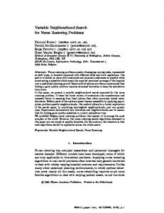
HM improvement. Due to the experience of unsatisfied solution in HM, N2 tends to increase a probability for randomly searching out of current design points. This also can provide new design points easier than others when compared. Finally, HM with searching rules from MSM is the final variant of HSA. N3 uses MSM to enhance a chance of the improvement probability in each iteration. In HM experience, the solutions are sorted from the best solutions to the worst solutions. These are used to determine possible vertices of expansion, reflection, contractions as N3. A pure interchange of HSA via N1, N2 and N3 will be performed for hybridisations of HSN1, HSN2 and HSN3, respectively. The three interchange of HSN4 attempts to shift among those three neighbourhoods. As appeared earlier on the literatures, each algorithm has its own influential parameters that affect its performance in terms of solution quality and execution time. To achieve the most preferable parameter choices that suit the tested problems, a large number of experiments were conducted. For each algorithm, an initial setting of the parameters was established using values previously reported in the literature. Then, the parameter values were changed one by one and the results were monitored in terms of the solution quality. The final parameter values adopted for each of the method are given in the following. For all optimisation problems presented in this paper, HSA parameters were set as follows: HMS = 20, PHMCR = 0.90, and PPAR = 0.35. For each model, the computational run using each algorithm was repeated 20 times. The experimental results obtained from each algorithm including best-so-far (BSF) solutions were compared for all models previously described. From the experimental results shown in Table 1, it suggested that HSA can produce an acceptable solution if the problem was not so complicated. HSA seems to get into trouble in operating local search for numerical applications of constrained response surface models. In order to improve the fine-tuning characteristic of HSA, HSA employs various procedures that enhance fine-tuning characteristic and convergence rate of HSA. The power of HSA with the fine tuning feature of mathematical tools is performed via four variants. Numerical results (Table 1) reveal that the proposed hybrid algorithms are powerful search algorithms for both unconstrained and constrained optimisation problems. New versions of HSA were dramatically better than those results obtained from the conventional when compared. They performed well at identifying the best-so-far (BSF) solutions at a reasonable execution time. The exploitation process via various hybridisations can be performed on each population member to improve its experience and thus obtain a population of local optimum solutions. The average execution time required by its hybridisations was also dramatically faster than the conventional HSA. When the problem is more complicated HSN4 is more suitable to exploit a solution space. It can be seen that these hybridisations on all models, except Shekel and constrained model III, were statistically significant itself with a 95% confidence interval (Table 2). Levels of the decision variables from the best so far results in each tested models are briefly given via HSA in Table 3. Results reported on tables are plotted on Fig. 4. Both from tables and figures, it can be said that the performance of HSA and HSN1-HSN3


algorithms are more sensitive to the increment in problem dimensions as compared to HSN4. 80.005

80

79.995

79.99

79.985

79.98

HSA HSN1 HSN2 HSN3 HSN4 Rosenbrock Model

79.975

79.97

79.965 1

10

100

1800 1600 1400 1200 1000 800 600

HSA HSN1 HSN2 HSN3 HSN4

400 200

Constrained Model III

0 1

10

100

1000

Fig. 4 Graphical Results for Rosenbrock and Constrained III Models. For a consideration of models in terms of response surface optimisation, the performance of HSN4 was better than the remaining methods. Moreover, the average design points for unconstrained tested models of parabolic and rosenbrock surfaces using HSN4 was approximately 20 points whilst 2000 points were averagely taken by HSA. Other words, the average design points towards the optimum taken by HSN4 were 60 times lower than design points required by the HSA. Moreover, it can be said HSN4 produced reasonable results even for high dimension spaces for constrained response surfaces. Another issue, a drawback of HSA variants, is that they employ BW and PPAR parameters [13]. These are very important parameters in fine-tuning of optimised solution vectors, and can be potentially useful in adjusting convergence rate of HSA variants towards the optimal solution. The variant of HSN3 applied the rules of contraction, reflection and expansion toward the optimum. It can cause the high performance of the algorithm and the considerable decrease in iterations needed to find the optimum. Furthermore, in some additional experiments, small BW values with large PPAR values usually cause the improvement of best solutions in final generations to converge to the optimal solution vector. When experimental results were analysed in terms of best solutions, it was found that HSA alone can produce an acceptable solution or even an optimal solution if the problem was not so complicated. When the problem is more complicated, the HSA variants are more suitable to exploit a search space by applying individuals’ experience of neighbourhood and then obtaining a population of local optimal solutions. REFERENCES [1]

K.S. Lee and Z.W. Geem, “A New Meta-heuristic Algorithm for Continuous Engineering Optimisation: Harmony Search Theory and Practice,” Comput: Meth. Appl. Mech. Eng., vol. 194, 2004, pp. 3902– 3933.

IMECS 2010


[2] [3]

[4]

[5]

[6]

[7]

[8]

P. Muller and D.R. Insua, “Issues in Bayesian Analysis of Neural Network Models,” Neural Computation, vol. 10, 1995, pp. 571–592. M. Dorigo, V. Maniezzo and A. Colorni, “Ant System: Optimisation by a Colony of Cooperating Agents,” IEEE Transactions on Systems, Man, and Cybernetics Part B, vol. 26, numéro 1, 1996, pp. 29-41. E. Emad, H. Tarek and G. Donald, “Comparison among Five Evolutionary-based Optimisation Algorithms,” Advanced Engineering Informatics, vol. 19, 2005, pp. 43-53. J.Y. Jeon, J.H. Kim and K. Koh, “Experimental Evolutionary Programming-based High-Precision Control,” IEEE Control Sys. Tech., vol. 17, 1997, pp. 66-74. R.Storn, “System Design by Constraint Adaptation and Deferential Evolution,” IEEE Trans. on Evolutionary Computation, vol. 3, no. 1, 1999, pp. 22-34. M. Clerc and J. Kennedy, “The Particle Swarm-Explosion, Stability, and Convergence in a Multidimensional Complex Space,” IEEE Transactions on Evolutionary Computation, vol. 6, 2002, pp.58-73.

HSA

HSN1

HSN2

HSN3

HSN4

Models BSF Mean Worst Standard Deviation BSF Mean Worst Standard Deviation BSF Mean Worst Standard Deviation BSF Mean Worst Standard Deviation BSF Mean Worst Standard Deviation

[9] [10]

[11]

[12]

[13]

A. Lokketangen, K. Jornsten and S. Storoy “Tabu Search within a Pivot and Complement Framework,” International Transactions in Operations Research, vol. 1, no. 3, 1994, pp. 305-316. N. Mladenovic and P. Hansen, “Variable Neighborhood Search,” Computers and Operations Research, vol. 24, 1997, pp. 1097–1100. P. Hansen and N. Mladenovic, “Variable Neighborhood Search: Principles and Applications,” European Journal of Operations Research, vol. 130, 2001a, 449–467. M. Mahdavi, M. Fesanghary and E. Damangir. “An Improved Harmony Search Algorithm for Solving Optimisation problems,” Applied Mathematics and Computation, vol. 188, 2007, pp. 1567–1579. W.G.R. Spendley, G.R. Hext and F.R. Himsworth, "Sequential Application of Simplex Designs in Optimisation and Evolutionary Operation," Technometrics, vol. 4, no. 4, 1962, pp. 441-461. V. Granville, M. Krivanek and J.P. Rasson, “Simulated Annealing: a Proof of Convergence”, Pattern Analysis and Machine Intelligence, IEEE Transactions, vol. 16, 1994, pp. 652 – 656.

TABLE 1: Experimental Results Obtained from Related Methods on each Tested Models Parabolic Rosenbrock Shekel Constrained I Constrained II Constrained III 12.0000 80.0000 18.9799 13.96110 -30647.3200 683.6144 12.0000 80.0000 18.9790 13.73859 -30639.8132 685.6502 12.0000 80.0000 18.9766 13.64373 -30633.6700 687.4941

Constrained IV -16.6535 -15.9389 -15.2724

0.0000

0.0000

0.0014

0.14943

6.7892

1.5034

0.5906

12.0000 12.0000 12.0000

80.0000 80.0000 80.0000

18.98051 18.98051 18.98051

13.63476 13.61740 13.59934

-30630.1526 -30627.0626 -30622.2983

685.4041 686.2882 687.7807

-17.0306 -16.5590 -16.1116

0.0000

0.0000

0.00000

0.01471

3.1219

0.9702

0.4411

12.0000 12.0000 12.0000

80.0000 80.0000 80.0000

18.98051 18.98051 18.98051

13.5914 13.5924 13.5939

-30651.6563 -30644.8912 -30636.2269

683.5490 685.3432 686.2891

-17.8706 -17.0475 -16.1116

0.0000

0.0000

0.00000

0.0012

6.4216

1.1958

0.7003

12.0000 12.0000 12.0000

80.0000 80.0000 80.0000

18.9799 18.9437 18.8020

13.6189 13.6497 13.7094

-30648.2087 -30646.3613 -30640.9764

684.7626 685.7400 686.2580

-17.1364 -16.7050 -16.1997

0.0000

0.0000

0.0792

0.0427

3.0711

0.6265

0.3562

12.0000 12.0000 12.0000

80.0000 80.0000 80.0000

18.98052 18.98051 18.98051

13.5908 13.5924 13.5931

-30665.2956 -30657.3340 -30651.1987

686.6879 686.8873 687.1560

-17.9198 -17.3333 -16.8832

0.0000

0.0000

0.00000

0.0011

5.2567

0.1981

0.4712

TABLE 2: Significant Effects on HSA and its Hybridisations (a) including Analysis of Variance (ANOVA) on Constrained Function IV (b) (a) Models Parabolic Rosenbrock Shekel Constrained I Constrained II Constrained III Constrained IV

Models

(b) P-Value N/A N/A 0.228519 0.005478 3.53E-07 0.160857 0.005545

Source of Variation Between Groups Within Groups Total

SS 5.597802 5.531149 11.12895

df 4 20 24

MS 1.399450 0.276557

F 5.060252

TABLE 3: Best So Far Results Obtained from HSA on each Tested Models Decision Variables x1

x2

x3

x4

x5

x6

x7

x8

P-Value 0.005545

Mean

Parabolic

0.0086

0.0044

12.0000

Rosenbrock

0.0123

-0.0291

80.0000

Shekel

5.9498

-6.9498

18.9805

Constrained I

2.2452

2.3626

13.6347

Constrained II

78.001

33.005

30.107

45.0

36.5

Constrained III

2.0396

2.01343

-0.0451

4.2734

-0.7265

1.1379

1.6495

Constrained IV

8.6076

9.6863

9.1304

0.2191

9.6533

0.742

1.8207


F crit 2.866081

-30647.3200 683.6144 1.2649

-16.6535

IMECS 2010