HYBRIDISING LOCAL SEARCH WITH BRANCH-AND-BOUND FOR CONSTRAINED PORTFOLIO SELECTION PROBLEMS Fang He1, 2 and Rong Qu1 1 The Automated Scheduling, Optimisation and Planning (ASAP) Group, School of Computer Science The University of Nottingham, Nottingham, NG8 1BB, UK 2 Department of Computer Science, Faculty of Science and Technology, University of Westminster, W1B 2HW, UK Email:
[email protected],
[email protected]
KEYWORDS Hybrid algorithm; Branch-and-Bound; local search; portfolio selection problems ABSTRACT In this paper, we investigate a constrained portfolio selection problem with cardinality constraint, minimum size and position constraints, and non-convex transaction cost. A hybrid method named Local Search Branch-and-Bound (LS-B&B) which integrates local search with B&B is proposed based on the property of the problem, i.e. cardinality constraint. To eliminate the computational burden which is mainly due to the cardinality constraint, the corresponding set of binary variables is identified as core variables. Variable fixing (Bixby, Fenelon et al. 2000) is applied on the core variables, together with a local search, to generate a sequence of simplified sub-problems. The default B&B search then solves these restricted and simplified subproblems optimally due to their reduced size comparing to the original one. Due to the inherent similar structures in the sub-problems, the solution information is reused to evoke the repairing heuristics and thus accelerate the solving procedure of the subproblems in B&B. The tight upper bound identified at early stage of the search can discard more subproblems to speed up the LS-B&B search to the optimal solution to the original problem. Our study is performed on a set of portfolio selection problems with non-convex transaction costs and a number of trading constraints based on the extended mean-variance model. Computational experiments demonstrate the effectiveness of the algorithm by using less computational time. INTRODUCTION In this paper, we tackle the single-period portfolio selection problem (PSP). In the problem concerned, a number of transactions can be carried out to adjust the portfolio during a given trading period. We take into account these transaction costs as well as a set of
trading constraints. These include the cardinality constraint (a limit on the total number of assets held in the portfolio, i.e. select k out n (k0 means buying. A weight w vectorr w denotes the portfolio affter the revission. After tthe transaction, tthe adjusted portfolio p is w = w0 + x, andd is held for a fixxed period of time. t We denote the returnn of asset i at the end of the innvestment periiod as ri and tthe expected retuurn of the poortfolio as R. We denote tthe covariance bbetween assetss i and j in return as σij. W We further defiine ( x ) as the sum of individuual transaction ccosts associateed with each xi. Based on tthe basic MV m model, the porttfolio selectio on problem w with transaction costs can thus be b modeled ass follows: i n j n
min
i 1 j 1
ij
wi w j (x)
(1)
i n
s.t.
ri wi R
(2)
w = w0 + x F
(3)
i 1
where objecctive (1) is to t minimize the risk of tthe portfolio andd the transaction costs incurrred. (2) ensurres the expected return. F in (3) ( represents a set of feasibble portfolios suubject to all thhe related constraints. Theese constraints iinclude the minimum m position size, tthe minimum traading size, etc., which will be b detailed neext. In this papeer, we modeel the probleem as a singgle
Fig.1 F The transaction cost fu function (Lobo o, Fazel et al. 20007) a Trading Prroblem Modeel with Transsaction Cost and Constraints Paarameter n
The tottal number off assets
i
The ind dex of assets, i=1,…,n
w0
Initial position p of thee portfolio
ij
Covariance betweenn assets i and j
ri
Return of asset i at thhe end of the investment period
R
Expectted return of thhe portfolio
i
Fixed cost c for buying ng or selling assset i
i
Variable cost rate foor buying or seelling asset i
There are two groups of variables in the formulation of the problem, as denoted by the “feature” column. wi, sell buy sell xibuy , xi are decision variables. zi , zi and zi are
wmin
Minimum hold position
xmin
Minimum trading amount
k
Number of assets in the portfolio after transaction
Variable
Feature
wi
Revised position of the portfolio after transaction
Decision variable
xibuy
Amount of buying asset i
Decision variable
xisell
Amount of selling asset i
Decision variable
auxiliary variables which are used to formulate the constraints. The column “core variable” denotes which variables are core variables. The selection of the core variables is problem dependent. Several researchers have pointed out that the cardinality constraint presents the greatest computational challenge to the problem (Bienstock 1996, Jobst, Horniman et al. 2001, Stoyan and Kwon 2010, Stoyan and Kwon 2011). Actually, the PSP with cardinality constraint has been recognized to be NP-complete (Bienstock 1996, Mansini and Speranza 1999). To eliminate the cardinality constraint, we identify variables zi which define the cardinality constraint
zi
Hold asset i or not in the revised portfolio
zibuy
Buy asset i or not
zisell
Sell asset i or not
i n j n
i n
i 1 j 1
i 1
min ij wi wj +i ( xi )
Auxiliary variable
i 1
i
k
as a set of core variables.
Based on the model PSP, we will introduce two Auxiliary variable additional reduced models (PSP basic, PSP sub) as follows which will be applied to evaluate the Auxiliary variable neighbourhood in the local search and to calculate the lower bound: (1)
(PSP)
in j n
min ij ww i j
(1)
st. .
i n
rw R i
(2)
i
wi w x
buy i
x , i 1,...n
in
rw R
(2)
i1
i i
sell i
(3)
wi zi , i 1,...n
(6)
w (x ) 1
(5)
wmin zi wi , i 1,...n
(7)
wi zi , i 1,...n
(6)
wmin zi wi , i 1,...n
(7)
0 i
i n i 1
i n
i
i
i 1
i
i n
zi k
in
(8)
i 1
xmin zibuy xibuy , i 1,...n x , i 1,...n
sell min i
sell i
x z
(9) (10)
xisell zisell , i 1,...n
(11)
xibuy zibuy , i 1,...n
(12)
zibuy zi , i 1,...n
(13)
buy i
z
(PSP basic)
i1 j 1
s.t. i 1
in
z
z
sell i
1 , i 1,...n
(14)
0 wi 1, i 1,...n
(15)
0 xibuy 1, i 1,...n
(16)
0 x
1, i 1,...n
(17)
zi , z , z {0,1}, i 1,...n
(18)
sell i
buy i
sell i
z k
(8)
0 wi 1, i 1,...n
(15)
i1
i
zi with assignments in {0,1}, i 1,...n (18) in jn
in
i1 j1
i1
minijww i j +i (xi )
(1)
st. . (2) (17) zwithassignments in {0,1},i 1,...n i
(18)
zibuy, zisell {0,1},i 1,...n
(19)
LS-B&B TO PSP ALGORITHM
(PSP sub)
In this section, we propose a new hybrid search, named LS-B&B to PSP according to the property of the problem. To the PSP with binary variable zi we are dealing with, we know that exactly k out n binary variables will be assigned to 1 in the feasible and optimal solutions. With this knowledge, we can apply variable fixing on a set of variables at one time, resulting into simplified sub-problem. A local search is performed on these set of variables to generate a sequence of sub-problems, and the best solution will be identified among them. Framework of LS-B&B to PSP
We present the framework of LS- B&B to PSP, as shown in Fig.2. LS-B&B consists of four main components. The first component is the initialization phase (line 1). In this phase, variable fixing is applied to the core variables to generate a simplified sub-problem. Lower bound and upper bound of the problem are also initialized in this phase. The second component is a default B&B search (line 7). It is called to solve the sub-problems to optimality. This solution to the sub-problem together with the variable assignments by variable fixing, forms the solution to the original problem. The third component is a local search (line 9) which is performed on set Z of variable zi to update sets S and. With the updated S, the sub-problem is updated correspondingly. Therefore, we state that this local search generates a sequence of sub-problems. The fourth component is an overall search procedure (the while loop). In this search procedure, a local search, variable fixing and a default B&B work together to identify the best solution among the subproblems by pruning inferior sub-problems and solving the promising sub-problems to optimality.
fix variables in subsets S to 1, to obtain sub-problems Psuby as follows: Psuby : min cT x s.t. Ax b; x j 1, j S B x j [0,1], j C
In this way, we simplify the original problem to a subproblem. One selection of the subsets S can generate one possible simplified sub-problem of the original problem. Therefore, we apply variable fixing together with a local search to generate a sequence of subproblems where we will search for the best solution. LS- B&B LB: lower bound; UB: upper bound; (h, x, w, z): a solution (x, w, z) of the problem with a corresponding objective value h; solveB&B: a default B&B solver; Z: set of zi; S: subset of Z; Porg: the original problem defined by model (PSP); Psub : sub-problem defined by variable fixing; y
1: Initialization phase 2: while (the number of iterations not met) 3: If (LB ( Psub ) ≥ UB) y
prune the sub-problem Psub ; y
4: 5: 6: 7: 8: 9:
go to line 9; Else (h, x, w, z) = solveB&B( Psub ) ; y
if h