Hybrid Local Search for Constrained Financial Portfolio Selection Problems Luca Di Gaspero1 , Giacomo di Tollo2 , Andrea Roli3 , and Andrea Schaerf1 1
DIEGM, Universit` a degli Studi di Udine, via delle Scienze 208, I-33100, Udine, Italy {l.digaspero | schaerf}@uniud.it 2 Dipartimento di Scienze, Universit` a “G.D’Annunzio”, viale Pindaro 42, I-65127, Pescara, Italy
[email protected] 3 DEIS, Alma Mater Studiorum Universit` a di Bologna, via Venezia 52, I-47023 Cesena, Italy
[email protected]
Abstract. Portfolio selection is a relevant problem arising in finance and economics. While its basic formulations can be efficiently solved through linear or quadratic programming, its more practical and realistic variants, which include various kinds of constraints and objectives, have in many cases to be tackled by approximate algorithms. In this work, we present a hybrid technique that combines a local search, as master solver, with a quadratic programming procedure, as slave solver. Experimental results show that the approach is very promising and achieves results comparable with, or superior to, the state of the art solvers.
1
Introduction
The portfolio selection problem consists in selecting a portfolio of assets that provides the investor a given expected return and minimises the risk. One of the main contributions in this problem is the seminal work by Markowitz [25], who introduced the so-called mean-variance model, which takes the variance of the portfolio as the measure of investor’s risk. According to Markowitz, the portfolio selection problem can be formulated as an optimisation problem over real-valued variables with a quadratic objective function and linear constraints. In this paper we consider the basic objective function introduced by Markowitz, and we take into account two additional constraints: the cardinality constraint, which limits the number of assets, and the quantity constraint, which fixes minimal and maximal shares of each asset included in the portfolio that force some specific assets to be included in the portfolio. For an overview of the formulations presented in the literature we forward the interested reader to [7]. We devise a hybrid solution based on a local search metaheuristic (see, e.g., [13]) for selecting the assets to be included in the portfolio, which at each step resorts to a quadratic programing (QP) solver for computing the best allocation for the chosen assets. The QP procedure implements the Goldfarb-Idnani dual algorithm [11] for strictly convex quadratic programs. The use of a hybrid solver has been (independently) proposed also by MoralEscudero et al. [26], who make use of genetic algorithms instead of local search for the determination of the discrete variables.
The paper is organised as follows: In Section 2 we introduce the problem formulation and in the following section (3) we succinctly review the most relevant works that describe metaheuristic techniques applied to formulations closely related to the one discussed in this paper. In Section 4 we present our hybrid solver detailing its components and Section 5 collects the results of the experimental analysis we performed. Finally, in Section 6, we draw some conclusions and point out our plans for further work.
2
Problem definition
Following Markowitz [25], we are given a set of n assets, A = {a1 , . . . , an }. Each asset ai has an associated real-valued expected return (per period) ri , and each pair of assets hai , aj i has a real-valued covariance σij . The matrix σn×n is symmetric and the diagonal elements σii represent the variance of assets ai . A positive value R represents the desired expected return. The values ri and σij are usually estimated from past data and are relative one fixed period of time. A portfolio is a vector of real values X = {x1 , . . . , xn }P such P that each xi n n represents the fraction invested in the asset ai . The value i=1 j=1 σij xi xj represents the variance of the portfolio, and is considered as the measure of the risk associated with the portfolio. Whilst the initial formulation by Markowitz [25] was a bi-objective optimisation problem, in many contexts financial operators prefer to tackle a single-objective version, in which the problem is to minimise the overall variance, ensuring the expected return R. The formulation of the basic (unconstrained) problem is thus the following.
min f (X) =
n X n X
s.t.
i=1 j=1 n X
(1)
i=1 n X
(2)
σij xi xj
ri xi ≥ R xi = 1
i=1
0 ≤ xi ≤ 1
(i = 1, . . . , n)
(3)
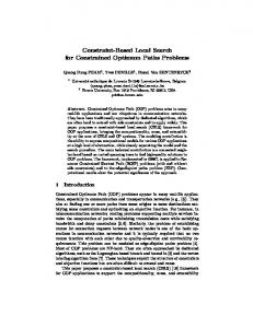
This is a quadratic programming problem, and nowadays it can be solved optimally using available tools despite the NP-completeness of the underlying decision problem [20]. Since R can be considered a parameter of the problem, solvers are usually compared over a set of instances, each with a specific value of minimum required expected return. By solving the problem as a function of R, ranging over a finite and discrete domain, we obtain the so-called unconstrained (Pareto) efficient frontier (UEF), that gives for each expected return the minimum associated risk. The UEF for one of the benchmark instances employed in this study is provided in Figure 1 (the lowest black solid line).
Fig. 1: Unconstrained and constrained efficient frontier.
Although the classical Markowitz’s model is extremely useful from the theoretical point of view, dealing with real-world financial markets imposes some additional constraints that are going to be considered in this work. In order to model them correctly, we need to add to the formulation a vector of n binary decision variables Z such that zi = 1 if and only if asset i is in the solution (i.e., xi > 0). Cardinality constraint: The number of assets that compose the portfolio is bounded: we give two values kmin and kmax (with 1 ≤ kmin ≤ kmax ≤ n) such that: n X zi ≤ kmax (4) kmin ≤ i=1
Quantity constraints: The quantity of each asset i that is included in the portfolio is limited within a given interval: we give a minimum ǫi and a maximum δi for each asset i, such that: xi = 0 ∨ ǫi ≤ xi ≤ δi
(i = 1, . . . , n)
(5)
Notice that the minimum cardinality constraints are especially meaningful in presence of constraints on the minimum quantity, otherwise they can be satisfied by infinitesimal quantities. We call CEF the analogous of the UEF for the constrained problem. In Figure 1 we plot the CEF found by our solver for the values ǫi = 0.01, δi = 1 (for i = 1, . . . , n), kmin = 1, and kmax varying from 4 to 12. For higher values of kmax the cardinality constraint reduces its effect and the curve is almost
indistinguishable from the UEF, indeed the distance among the CEF and UEF4 becomes smaller than 10−3 for the instance at hand. Constraints 4 and 5 make it intractable to solve real-world instances of problem with proof of optimality [14]. Therefore, either simplified models considered, such as formulations with linear objective function [21, 22], or proximate methods are applied.
3
the the are ap-
Related work
Local search approaches have been widely applied to portfolio selection problems under many different formulations. The first work on this subject appearing in the literature is due to Rolland [30], who presents an implementation of Tabu Search to tackle the unconstrained formulation. This formulation is considered also in the implementation of evolutionary techniques in [2, 18, 19]. The use of local search techniques for the constrained portfolio selection problem has been proposed by several authors, including Chang et al. [4], Gilli and K¨ellezi [9] and Schaerf [31]. The cited works however use local search as a monolithic solver, exploring a search space composed of both continuous and discrete variables. Conversely, our hybrid solver focuses on the discrete variables, leaving the determination of the continuous ones to the QP solver. In addition, we consider here a more general problem w.r.t. the cited three papers, including also the possibility to specify a minimum number of assets (and not only the maximum). Among the population-based methods developed for tackling the constrained formulation, we mention Streichert et al. [33], in which the cardinality constrained variant is considered, and memetic algorithm approaches introduced in [12, 15, 24]. These strategies, by being inherently effective in diversifying the search, exhibit good performance especially in multi-objective formulations, as shown by the family of Multi-Objective Evolutionary Algorithms [17, 8, 27, 33]. Finally, Ant Colony Optimisation has also been successfully applied to portfolio problems modelled with the cardinality constraint in [1, 23]. For the sake of completeness, we also mention interesting hybrid heuristic techniques based on linear programming that have been introduced in [32] and deal with a linear objective function formulation with integer variable domains. In this case, the value assigned to a variable represents the actual amount invested in the asset. The basic idea behind these approaches is to relax the discrete constraint on quantities, transforming the problem into a linear programming problem and find a solution to it. Fractional asset weights are then rounded to the closest admissible discrete quantity and a possible infeasible solution is repaired heuristically. More robust strategies use the solution to the continuous relaxation to feed a mixed integer-linear programming solver [16, 20]. 4
Measured by what we call average percentage loss, introduced in Section 5.1.
4
A hybrid local search solver for portfolio selection
Our master solver is based on local search, which works on the space induced by the vector Z only. For computing the actual quantities X, it invokes the QP (slave) solver, using as the input assets only those such that zi = 1 in the current state. In order to apply local search techniques we need to define the search space, the cost function, the neighbourhood structures, and the selection rule for the initial solution. 4.1
Search space and cost function
The search space is composed of the all 2n possible configurations of Z, with the exception of assignments that do not satisfy Constraints (4). These constraints are therefore implicitly enforced by the local search solver by excluding them from the search space. On the contrary, states that violate Constraints (1), (2), (3), or (5) are included, and these constraints are passed to the QP solver that handles them explicitly. The QP solver receives as input only those assets included in the state under consideration, and it produces the assignment of values to the corresponding xi variables. For all assets ai that are not included in the state we obviously set xi = 0. In addition, the QP solver also returns the computed risk f for the solution produced, which represents the cost of the state. If the QP solver is unable to produce a feasible solution it returns the special value f = +∞ (and the values xi returned are not meaningful). In this case, we relax Constraint (1) and we build the configuration, using only the assets included that gives the highest return without violating the other constraints. This construction is done by a greedy algorithm that sorts the assets by the expected return and assigns the maximum quantity to each asset in turn, as long as the sum is smaller than 1. In the latter case the cost is the degree of violation of Constraint (1) multiplied by a suitably large constant (that ensures that return related costs are always bigger than risk related ones). 4.2
Neighbourhood structure
The neighbourhood relation we propose is based on addition, deletion and replacement of an asset. A move m is identified by a pair hi, ji, where ai is the asset to be added and aj is the asset to be deleted (i, j ∈ {1, . . . , n}). The value of i can also be 0, meaning that no asset is added. Analogously for j, if j = 0 it means that no asset is deleted. Notice that not all pairs m = hi, ji, with i, j ∈ {0, 1, . . . , n}, correspond to a feasible move, since some values are meaningless, e.g. inserting an asset already present or setting both i and j to zero (null move). Moreover, moves that violates Constraints (4) are also considered infeasible, e.g. a delete move when the number of assets is equal to the minimum.
4.3
Initial solution construction
For the initial solution, we use three different strategies, that are employed at different stages of the search (as explained in Section 4.4). For all three, we ensure that Constraints (4) are always satisfied. RandomCard: We draw at random a number k (between kmin and kmax ), and we insert k randomly selected assets. MaxReturn: We build the portfolio that produces the maximum possible return (independently of the risk) PreviousPoint: We use the final solution of the previously computed point of the frontier 4.4
Local search techniques
We implemented three local search techniques, namely Steepest Descent (SD), First Descent (FD), and Tabu Search (TS). The SD strategy relies on the exhaustive exploration of the neighbourhood and the selection of the neighbour that has the minimal value of f (breaking ties at random). The SD strategy stops as soon as no improving move is available, i.e., when a local minimum has been reached. FD behaves as SD with the difference that, as soon as an improving move is found, it is selected and the exploration of the current neighbourhood is interrupted. For TS we use a dynamic-size tabu list to implement a short term prohibition mechanism and the standard aspiration criterion [10]. Like for SD, we search for the next state by exploring the full neighbourhood (excluding infeasible moves) at each iteration. In order to make the solvers more robust, for all techniques, we make two runs for each value of R: one using the RandomCard initial solution construction, and the other one starting from the best of the previous point (PreviousPoint initial solution). For the very first point of the frontier (highest requested return and no previous point available) we use instead the MaxReturn construction.
5
Experimental analysis
In this section, we first present the benchmark instances and the settings of our solver. In the following subsections, we show the comparison with all the previous works that use the same formulation. We conclude showing a search space analysis that tries to explain the behaviour of our solvers on the proposed instances. 5.1
Benchmark instances
We experimented our techniques on two groups of instances obtained from real stock markets and used in previous works. The first is a group of five instances
Inst. Origin
assets
UEF
Group 1 1 2 3 4 5
Hong Kong Germany UK USA Japan
31 85 89 98 225
1.55936 0.412213 0.454259 0.502038 0.458285
·10−3 ·10−3 ·10−3 ·10−3 ·10−3
Group 2 S1 USA (DataStream) 20 4.812528 S2 USA (DataStream) 30 8.892189 S3 USA (DataStream) 151 8.64933 Table 1: The benchmark instances.
taken from the repository ORlib available at the URL http://mscmga.ms.ai. ac.uk/∼jeb/orlib/portfolio.html. These instances have been proposed by Chang et al. [4] and have been studied also in [1, 26, 31]. The second group of three instances have been provided to us by M. Schyns and are used in [5]. For the first group, a discretised UEF composed of 100 equally distributed values for the expected return R is provided along with the data. For the second group, we computed the discretised UEF ourselves using the QP solver with all assets available and no additional constraints. As in previous works, we evaluate the quality of our solutions employing an aggregate indicator that measures the deviation of the CEF found by the algorithms w.r.t. the UEF on the whole set of frontier points. We call this measure average percentage loss (apl ) and we define it as follows: let Rl be the expected return, V (Rl ) and VU (Rl ) the values of the function f returned by the solver and the risk on the UEF, respectively, and l = 1, . . . , p where p is the P number of points of the frontier; the average percentage loss is equal to p 100 l=1 (V (Rl ) − VU (Rl ))/VU (Rl ). Table 1 illustrates for all instances the origp inal market, and the average variance of the UEF. 5.2
Experimental Setting of the Solvers
Experiments were performed on an Apple iMac computer equipped with an Intel Core 2 Duo (2.16 GHz) processor and running Mac OS X 10.4; the SD, FD and TS metaheuristics have been coded in C++ exploiting the framework EasyLocal++ [6], the QP solver has also been coded in C++ and is made publicly available from one of the authors’ website5 . The executables were obtained using the GNU C/C++ compiler (v. 4.0.1). Concerning the algorithms setting, SD and FD have no parameter to be set; for TS we tuned its parameters by means of a statistical technique called Frace [3] and found that the algorithm is very robust with respect to parameter 5
http://www.diegm.uniud.it/digaspero/
setting. We set the tabu list size in the range [3 . . . 10] and we stop the execution of TS when a maximum of 100 iterations without improvement was reached. 5.3
Comparison with previous results
Due to the different formulations employed by the authors, the only papers we can compare with are those of Schaerf [31] and Moral-Escudero et al. [26], who employ the same set of constraints on the ORlib instances, and with Crama and Schyns [5] who deal with a slightly different setting and with a novel set of instances. Concerning Chang et al. [4], as already pointed out in [31], even though they work on the ORlib instances (and with the same constraints), a fair comparison with their solutions is not possible because the problem is solved by taking points along the frontier that are not homogeneously distributed. Arma˜ nanzas and Lozano [1] work on a variant of the problem for which the values kmin and kmax coincide (i.e., kmin = kmax = K) on the ORlib instances. However, due to what we believe is an error in the implementation of their solution methods 6 they obtain a set of points that are infeasible w.r.t. Constraint (2). In details, they assign to the assets i for which zi = 1 chosen by their ACO algorithm the quantity xi = (δi − ǫi )/K, Pn therefore since they set ǫi = 0.001, δi = 1 for all i = 1, . . . , n, they obtain i=1 xi = 0.999 instead of 1. For this reason we could not compare our solvers with [1], nevertheless we are going to present some results on the behaviour of one of our solvers on the formulation proposed in that paper. Comparison with Schaerf [31] and Moral-Escudero et al. [26] For this comparison, we set the constraint values exactly as in [26, 31]: ǫi = 0.01 and δi = 1 for i = 1, . . . , n, and kmax = 10 for all instances. The minimum cardinality is not considered in the cited work, and therefore we set it to kmin = 1 (i.e., no limitation). Table 2 shows best results and running times obtained by our three solvers in comparison with previous work. Since Moral-Escudero et al. [26] report only the best outcomes of their solvers, in order to fairly compare with them we have to present the results as the minimum average percentage loss w.r.t. the UEF found by the algorithm. The results of our solvers are the best CEFs found in 30 trials of the algorithm on each instance and the running times reported are those of the best trial (exactly as in [26]). Running times of [31] are obtained re-running Schaerf’s software on our machine, those of Moral-Escudero et al. are taken from their paper, and are obtained using a PC having about the same performances. Table 2 shows that we obtain results superior to [31] both in terms of risk and running times. This suggests that the hybrid solver outperforms monolithic local search ones. Regarding [26], we obtain with SD exactly the same results of their best solver, but in a much shorter time (on a comparable machine). 6
We found the error in our analysis of the data provided to us by J. Lozano.
FD + QP SD + QP TS + QP GA + QP [26] TS [31] Inst. min apl time min apl time min apl time min apl time min apl time 1 0.00366 1.3s 0.00321 4.3s 0.00321 17.2s 0.00321 415.1s 0.00409 251s 2 2.66104 5.3s 2.53139 20.3s 2.53139 61.3s 2.53180 552.7s 2.53617 531s 3 2.00146 5.4s 1.92146 23.6s 1.92133 69.5s 1.92150 886.3s 1.92597 583s 4 4.77157 7.6s 4.69371 27.6s 4.69371 80.0s 4.69507 1163.7s 4.69816 713s 5 0.24176 15.7s 0.20219 69.5s 0.20210 210.7s 0.20198 1465.8s 0.20258 1603s Table 2: Comparison of results with Schaerf [31] and Moral-Escudero et al. [26].
As already pointed out in [31], even though Chang et al. [4] solve the same instances (and with the same constraints), a fair comparison with their solutions is not possible. This is because they consider the CEF differently. Specifically, they do not solve a different instance for each value of R, but (following Perold [28]), they reformulate the problem without Constraint (1) and with the following objective function: f (X) = λf1 (X) + (1 − λ)f2 (X). The problem is then solved for different values of λ, and what they obtain is the solution for a set of values for R which are not homogeneously distributed.
Comparison with Crama and Schyns [5] Since the results of Crama and Schyns [5] are presented in graphical form and make use of a slightly different cost function (i.e., they consider the standard deviation instead of the variance as the risk measure) we re-run their solver7 on the three instances employed in their experimentation employing the same parameter setting reported in their paper. The constraints set in this experiment are as follows: kmin = 1, kmax = 10, ǫi = 0, and δi = 0.25. In Table 3 we present the outcome of this comparison. For each algorithm we report in three columns the average and the standard deviation (in parentheses) of the average percentage loss w.r.t. the UEF, and the average time spent by the algorithm. The data was collected by running 30 times each algorithm on each instance and computing the whole CEF. From the table it is clear that, in terms of solution quality, the family of our solvers outperforms the SA approach of Crama and Schyns. Looking at the times, we can see that SA, in general, exhibits shorter running times than our hybrid SD and TS approaches. This can be explained by the strategy employed by both our algorithms that thoroughly explore the full neighbourhood of each solution whereas the SA randomly picks out only some neighbours thus saving time in the evaluation of the cost function. Moreover, the slave QP procedure is more time-consuming than the solution evaluation carried out by Crama and Schyns, however it allows us a higher accuracy on the assignment of the assets. 7
The executable was kindly provided to us by M. Schyns.
Inst.
FD + QP apl time
SD + QP apl time
TS + QP apl time
SA [5] apl time
S1 0.72 (0.094) 0.3s 0.35 (0.0) 1.4s 0.35 (0.0) 4.6s 1.13 (0.13) 3.2s S2 1.79 (0.22) 0.5s 1.48 (0.0) 3.1s 1.48 (0.0) 8.5s 3.46 (0.17) 5.4s S3 10.50 (0.51) 10.2s 8.87 (0.003) 53.3s 8.87 (0.0003) 124.3s 16.12 (0.43) 30.1s
15
20
25
30
k_min = 1, k_max = K k_min = k_max = K
0
0
5
10
40
60
average percentage loss
80
k_min = 1, k_max = K k_min = k_max = K
20
average percentage loss
35
Table 3: Comparison of results with Crama and Schyns [5].
0
10
20
30
40
K
(a) Results on instance 2.
50
10
20
30
40
K
(b) Results on instance 5.
Fig. 2: Average percentage loss found by our SD + QP solver varying K.
Results for fixed cardinality portfolios As mentioned previously, even though we cannot compare our results with the work of Arma˜ nanzas and Lozano [1], we decided to show some results of the SD solver on the ORlib instances by setting the cardinality constraints so that they force the constructed portfolio to have exactly kmin = kmax = K assets as in [1]. The quantity constraints are set as in the first set of experiments, i.e. ǫi = 0.01, and δi = 1. In Figure 2 we plot the behaviour of the average percentage loss found by our SD + QP solver at different values of K on a selected pair of instances. The curve is compared with the average percentage loss computed by the same solver but relaxing the minimum cardinality constraint to kmin = 1 (i.e., just allowing to include an increasing number of assets in the portfolios, but not obliging the solver to compel to a fixed cardinality). From the pictures we can notice an interesting phenomenon: the two curves are almost indistinguishable up to a value of K for which the fixed cardinality solutions tend to have an higher average percentage loss. In a sense, this sort of minimum represent the best compromise in the cardinality, i.e., the optimal fixed number of assets K that minimises the deviation from the best achievable returns (i.e, the UEF values).
5.4
Search space analysis
We study the search space main characteristics of the instances composing the benchmarks with the aim of providing an explanation for the observed algorithm behaviour and elaborating some guidelines for understanding the hardness of an instance when tackled with our hybrid local search. Once cardinality constraints are set, in general we are interested in studying the characteristics of the search space of the single instances of the problem along the frontier, i.e., at fixed values of return R. Among the 100 points composing the frontier, we took five samples homogeneously distributed along the frontier, in order to estimate the characteristics of the search spaces encountered by our solver along the whole frontier. Moreover, constrained instances with different values of kmin and kmax have been considered. In our experiments, we chose (kmin , kmax ) ∈ {(3, 3), (6, 6), (10, 10), (1, 3), (1, 6), (1, 10)}. One of the most relevant search space characteristics is the number of global and local minima. The number of local minima is usually taken as an estimation of the ruggedness of the search space, that, in turn, is roughly negatively correlated with local search performance [13]. In order to estimate the number of minima in an instance, we run a deterministic version of SD (called SDdet )8 starting from initial states either produced by complete enumeration (for very small size instances) or by uniformly sampling the search space. Our analysis shows that the instances of the benchmarks have a very small number of local minima, and only one global minimum (i.e., either a certified global minimum, when exhaustive enumeration is performed, or the best known solution, otherwise). Most of the analysed instances have only one minimum and the other instances have not more than six minima. We observed that the latter cases occur usually at low values of return R. Instance 4 is the one with the greatest number of local minima, while the remaining instances have very few cases with local minima. This analysis may provide an explanation for the very similar performance exhibited by SD and TS in terms of solution quality. To strengthen this argument, we also studied global and local minima basins of attraction, in order to estimate the probability of reaching a global minimum [29]. Given a deterministic algorithm such as SDdet , the basin of attraction B(s) of a minimum s, is defined as the set of states that, taken as initial states, give origin to trajectories that ends at point s. The cardinality of B(s) represents its size (in this context, we always deal with finite spaces). The quantity rBOA(s), defined as the ratio between the size of B(s) and the search space size, is an estimation of the reachability of state s. If the initial solution is chosen at random, the probability of finding a global optimum s∗ is exactly equal to rBOA(s∗ ). Therefore, the higher is this ratio, the higher is the probability of success of the algorithm. Both SD and TS incorporate stochastic decision mechanisms and TS is also able to escape from local minima, therefore the estimation of basins of attraction size related to SDdet provides a lower bound on the probability of reaching the global optimum when using SD and TS. 8
Ties are broken by enforcing a lexicographic order of states.
risk
0.000160
0.000162
0.000164
0.000320 0.000316
risk 0.000312 0.000308 0.0
0.2
0.4
0.6
0.8
0.0
1.0
0.2
0.4
0.8
1.0
(b) Instance 4: kmin = 1, kmax = 6, R = 0.0019368822.
risk
1.090
0.0001790
1.095
1.100
risk
1.105
0.0001794
1.110
(a) Instance 4: kmin = kmax = 3, R = 0.0037524115.
0.6
rBOA
rBOA
0.0
0.2
0.4
0.6
0.8
1.0
rBOA
(c) Instance 4: kmin = 1, kmax = 10, R = 0.0037524115.
0.0
0.2
0.4
0.6
0.8
1.0
rBOA
(d) Instance S3: kmin = 1, kmax = 6, R = 0.260588.
Fig. 3: Basins of attraction of minima on two benchmark instances with different cardinality and return constraints.
The outcome of our analysis is that global minima have usually a quite large basin of attraction. Representative examples of these results are depicted in Figures 3a, 3b, 3c and 3d; segments represent the basins of attraction: their length corresponds to rBOA and their y-value is the objective value of the corresponding minimum. We can note that global minima have a quite large basin of attraction whose rBOA ranges from 30% (in Figure 3c) to 60% (in Figure 3a). It is worth remarking that these large basins are specific for our hybrid solver, and this is not the case for monolithic local search ones. The presence of large basins of attraction for the global optimum suggests that the best strategy for tackling these instances is simply to run SD with random restarts, and that there is no need for a more sophisticated solver such as TS. However, since TS has better exploration capabilities than SD, it could still show superior performances on other, possibly more constrained, instances. Indeed, it is possible construct artificial instances with a large number of local minima and a small basin for the global one; it is straightforward to show that for such instances TS performs much better than SD for all values of R.
6
Conclusions and future work
Experiments show that our solver is comparable with (or superior to) the state of the art for the less constrained problem formulation (no minimum). Comparison for the general problem are subject of ongoing work. In the future, we plan to adapt this approach to tackle other formulations, such as the discrete formulation that is particularly interesting for some investors. This formulation enables us to take into account aspects of real-world finance, such as transaction costs. To this extent, instances including minimum lots will be investigated, since assets generally cannot be purchased in any quantity and the amount of money to be invested in a single asset must be a multiple of a given minimum lot [20]. Moreover, we are going to include also asset preassignments, that will be useful for representing investor’s subjective preferences. We also aim at identifying difficult instances and verify whether more sophisticated local search metaheuristics, such as TS, could improve on the results of the simple SD strategy.
Acknowledgements We thank Jose Lozano, Renata Mansini, Michael Schyns, and Ruben RuizTorrubiano for helpful clarification about their work.
References [1] R. Arma˜ nanzas and J.A. Lozano. A multiobjective approach to the portfolio optimization problem. In Proceedings of the 2005 IEEE Congress on Evolutionary Computation (CEC 2005), volume 2, pages 1388–1395. IEEE Press, 2005. doi: 10.1109/CEC.2005.1554852. [2] S. Arnone, A. Loraschi, and A. Tettamanzi. A genetic approach to portfolio selection. Neural Network World – International Journal on Neural and Mass-Parallel Computing and Information Systems, 3(6):597–604, 1993. [3] M. Birattari, T. St¨ utzle, L. Paquete, and K. Varrentrapp. A racing algorithm for configuring metaheuristics. In W. B. Langdon et al., editor, Proceedings of the Genetic and Evolutionary Computation Conference (GECCO 2002), pages 11–18, New York, 9–13 July 2002. Morgan Kaufmann Publishers. [4] T.-J. Chang, N. Meade, J. E. Beasley, and Y. M. Sharaiha. Heuristics for cardinality constrained portfolio optimisation. Computers & Operations Research, 27(13):1271–1302, 2000. [5] Y. Crama and M. Schyns. Simulated annealing for complex portfolio selection problems. European Journal of Operational Research, 150:546–571, 2003. [6] L. Di Gaspero and A. Schaerf. EasyLocal++: An object-oriented framework for flexible design of local search algorithms. Software—Practice & Experience, 33(8):733–765, 2003.
[7] G. di Tollo and A. Roli. Metaheuristics for the portfolio selection problem. Technical Report R-2006-005, Dipartimento di Scienze, Universit` a “G. D’Annunzio” Chieti–Pescara, 2006. [8] L. Dio¸san. A multi-objective evolutionary approach to the portfolio optimization problem. In Proceedings of the International Conference on Computational Intelligence for Modelling, Control and Automation (CIMCA 2005), pages 183–188. IEEE Press, 2005. [9] M. Gilli and E. K¨ellezi. A global optimization heuristic for portfolio choice with VaR and expected shortfall. In P. Pardalos and D.W. Hearn, editors, Computational Methods in Decision-making, Economics and Finance, Applied Optimization Series. Kluwer Academic Publishers, 2001. [10] F. Glover and M. Laguna. Tabu search. Kluwer Academic Publishers, 1997. [11] D. Goldfarb and A. Idnani. A numerically stable dual method for solving strictly convex quadratic programs. Mathematical Programming, 27:1–33, 1983. [12] M.A. Gomez, C.X. Flores, and M.A. Osorio. Hybrid search for cardinality constrained portfolio optimization. In Proceedings of the 8th annual conference on Genetic and Evolutionary Computation,, pages 1865–1866. ACM Press, 2006. doi: 10.1145/1143997.1144302. [13] H.H. Hoos and T. St¨ utzle. Stochastic Local Search Foundations and Applications. Morgan Kaufmann Publishers, San Francisco, CA (USA), 2005. ISBN 1-55860-872-9. [14] N.J. Jobst, M.D. Horniman, C.A. Lucas, and G. Mitra. Computational aspects of alternative portfolio selection models in the presence of discrete asset choice constraints. Quantitative Finance, 1:1–13, 2001. [15] H. Kellerer and D.G. Maringer. Optimization of cardinality constrained portfolios with a hybrid local search algorithm. OR Spectrum, 25(4):481– 495, 2003. [16] H. Kellerer, R. Mansini, and M.G Speranza. On selecting a portfolio with fixed costs and minimum transaction lots. Annals of Operations Research, 99:287–304, 2000. [17] D. Lin, S. Wang, and H. Yan. A multiobjective genetic algorithm for portfolio selection. Working paper, 2001. [18] A. Loraschi and A. Tettamanzi. An evolutionary algorithm for portfolio selection within a downside risk framework. In C. Dunis, editor, Forecasting Financial Markets, Series in Financial Economics and Quantitative Analysis, pages 275–285. John Wiley & Sons, Chichester, UK, 1996. [19] A. Loraschi, A. Tettamanzi, M. Tomassini, and P. Verda. Distributed genetic algorithms with an application to portfolio selection problems. In D. W. Pearson, N. C. Steele, and R. F. Albrecht, editors, Proceedings of the International Conference on Artificial Neural Networks and Genetic Algorithms, pages 384–387. Springer-Verlag, 1995. [20] R. Mansini and M.G. Speranza. Heuristic algorithms for the portfolio selection problem with minimum transaction lots. European Journal of Operational Research, 114:219–233, 1999.
[21] R. Mansini and M.G. Speranza. An exact approach for portfolio selection with transaction costs and rounds. IIE Transactions, 37:919–929, 2005. [22] R. Mansini, W. Ogryczak, and M.G. Speranza. Lp solvable models for portfolio optimization a classification and computational comparison. IMA Journal of Management Mathematics, 14:187–220, 2003. [23] D.G. Maringer. Optimizing portfolios with ant systems. In Proceedings of the International ICSC congress on computational intelligence: methods and applications (CIMA 2001), pages 288–294. ISCS Academic Press, 2001. [24] D.G. Maringer and P. Winker. Portfolio optimization under different risk constraints with modified memetic algorithms. Technical Report 2003– 005E, University of Erfurt, Faculty of Economics, Law and Social Sciences, 2003. [25] H. Markowitz. Portfolio selection. Journal of Finance, 7(1):77–91, 1952. [26] R. Moral-Escudero, R. Ruiz-Torrubiano, and A. Su´ arez. Selection of optimal investment with cardinality constraints. In Proceedings of the IEEE World Congress on Evolutionary Computation (CEC 2006), pages 2382– 2388, 2006. [27] C.S. Ong, J.J. Huang, and G.H. Tzeng. A novel hybrid model for portfolio selection. Applied Mathematics and Computation, 169:1195–1210, October 2005. [28] A.F. Perold. Large-scale portfolio optimization. Management Science, 30 (10):1143–1160, 1984. [29] S. Prestwich and A. Roli. Symmetry breaking and local search spaces. In Proceedings of the 2nd International Conference on Integration of AI and OR Techniques in Constraint Programming for Combinatorial Optimization Problems (CP-AI-OR 2005), volume 3524 of Lecture Notes in Computer Science. Springer–Verlag, 2005. [30] E. Rolland. A tabu search method for constrained real-number search: applications to portfolio selection. Working paper, 1996. [31] A. Schaerf. Local search techniques for constrained portfolio selection problems. Computational Economics, 20(3):177–190, 2002. [32] M.G. Speranza. A heuristic algorithm for a portfolio optimization model applied to the Milan stock market. Computers & Operations Research, 23 (5):433–441, 1996. ISSN 0305-0548. [33] F. Streichert, H. Ulmer, and A. Zell. Comparing discrete and continuous genotypes on the constrained portfolio selection problem. In Proceedings of the Genetic and Evolutionary Computation Conference (GECCO 2004), volume 3103 of Lecture Notes in Computer Science, pages 1239–1250, Seattle, Washington, USA, 2004. Springer-Verlag.