Hydrodynamic approach to time-dependent density functional theory ...

arXiv:cond-mat/0003152v3 5 Jul 2000

Hydrodynamic approach to time-dependent density functional theory; response properties of metal clusters Arup Banerjee and Manoj K. Harbola Laser Programme, Centre for Advanced Technology, Indore 452013, INDIA. February 1, 2008 Abstract Performing electronic structure calculations for large systems, such as nanoparticles or metal clusters, via orbital based Hartree-Fock or Kohn-Sham theories is computationally demanding. To study such systems, therefore, we have taken recourse to the hydrodynamic approach to time-dependent density-functional theory. In this paper we develop variation-perturbation method within this theory in terms of the particle and current densities of a system. We then apply this to study the linear and nonlinear response properties of alkali metal clusters within the spherical jellium background model.

1

I Introduction The hydrodynamic analogy of quantum mechanics was first explored by Madelung [1] who transformed the single particle Schrodinger equation into a pair of hydrodynamical equations. The theory views [2, 3] the electron cloud as a classical fluid moving under the action of classical Coulomb forces augmented by the forces of quantum origin. The basic dynamical variables of this theory are the particle and current densities which satisfy two fluid dynamical equations, namely, the continuity and an Euler type equation. The work of Madelung was followed by Bloch’s attempt [4] to develop hydrodynamical theory for many-electron systems within the realm of Thomas-Fermi (TF) theory [5, 6, 7]. Although then proposed without any rigorous foundation, the theory can now be derived [8] from the equations of time-dependent density-functional theory (TDDFT) [9, 10]. It is based on the assumption that the dynamics of many-electron system can be described by considering it as a fluid of density ρ(r, t) and a velocity field v(r, t) which is assumed to be curl free (that is v(r, t) = −∇S(r, t), where S(r, t) is scalar velocity

potential). Using ρ(r, t) and S(r, t) as conjugate variables Bloch derived two fluid dynamical equations: the continuity equation ∂ρ + ∇ · (ρ∇S) = 0, ∂t

(1)

Z ∂S 1 δT0 ρ(r′ , t) ′ = |∇S|2 + + vext (r, t) + dr . ∂t 2 δρ |r − r′ |

(2)

and the Euler equation

Here T0 is the TF kinetic energy (KE) functional and vext (r, t) represents the external potential. These equations were subsequently used to study photoabsorption cross section and collective excitation of atoms[11], collective excitations [12] and plasmons of metal clusters [13] and surface plasmons [14, 15] in metals. 2

Bloch’s theory also formed the basis of initial attempts by Ying [16] to extend density-functional theory (DFT) to include time-dependent (TD) external potentials. He did this by replacing the TF KE term T0 by a general functional G[ρ] consisting of the KE and the exchange-correlation (XC) contribution to the total energy. In Ying’s work it is implicit that, like in the static DFT, a universal functional G[ρ(r, t)] can be written for the TD problem. The ad-hoc nature of Bloch’s theory and its extension by Ying was removed by the pioneering works of Deb and Ghosh [17], Bartolotti [18] and Runge and Gross [19]. Runge and Gross rigorously proved the existence of a Hohenberg-Kohn [20] like theorem for TD potentials, and showed that the TD density ρ(r, t) can be determined by solving the hydrodynamical equations

∂ρ + ∇ · j = 0, ∂t which is the continuity equation, and the Euler’s equation ∂j = P[ρ(r, t)]. ∂t

(3)

(4)

Here P is the three-component density-functional of Runge and Gross and the vector j is the current density corresponding to the many-body wavefunction Ψ(r1 , · · · , rN ; t). An explicit expression for P[ρ(r, t)] in terms of

the wavefunction has recently been given [8] using the TD differential virial theorem[21].

Although there have been some calculations, as mentioned above, in the past by employing hydrodynamic theory, its full potential remains unexplored. This is evidently because with the increasing computing resources one can perform [22] orbital based calculations like TD Hartee-Fock (HF) or TD Kohn-Sham (KS) with relative ease. Recently, however, hydrodynamical theory is being applied in situations where such orbital based calculations are still computationally difficult to implement. One such example is systems which contain thousands of atom such as nanoparticles and clusters. In these systems hydrodynamical theory becomes the method of choice. Thus 3

the theory has been applied to study photoabsorption cross-section of metal particles [23], collective [24] and magnetoplasmon excitations [25] of confined electronic systems and also to study the interaction of strong laser light with atomic systems [26, 27, 28]. Besides the computational ease offered by it, one is also tempted to work within the hydrodynamic formulation because it provides an intuitively appealing approach to the time dependent many-body problem. In this paper we develop perturbation theory within the hydrodynamic formalism to calculate linear and nonlinear response properties of large systems. The motivation for this comes from our experience with the calculation of static response properties [29, 30] employing density based perturbation theory [31] within the Hohenberg-Kohn formalism of DFT. The density based method reduces the numerical effort required for such calculations substantially while leading to reasonably accurate results [29, 30] for the response properties. In the same manner, the hydrodynamical approach proves to be useful for calculating frequency dependent response properties of extended systems for which orbital based theories become quite difficult to implement because of the large number of orbitals involved. The work presented in this paper is divided into two parts: First, we derive the generalized Bloch type equation using the concept of time-averaged energy (quasi-energy) of an electronic system subjected to a TD periodic field. For calculating optical response properties we then develop variationperturbation (VP) theory in terms of the quasi-energy using particle and current densities as the basic variables. This is presented in section II. The perturbation theory developed here proceeds along the lines of density based stationary-state perturbation theory [31] by making use of the stationary nature of the time-averaged energy with respect to ρ(r, t) and S(r, t). In the second part we demonstrate the applicability of the perturbation theory developed here by calculating frequency dependent linear and nonlinear polarizabilities of inert gas atoms (section III) and comparing our numbers

4

with the standard results obtained from the wavefunctional approach. Having demonstrated the accuracy of hydrodynamical approach, we then apply it to calculate frequency dependent response properties of metal clusters with number of atoms up to 5000 using the spherical jellium background model (SJBM).

II Variation perturbation method in hydrodynamical theory A. Time-averaged energy The central quantity around which the VP theory is developed in the static case is the ground-state energy of the system. For periodic TD hamiltonians, this role is played by the time-averaged energy or quasi-energy [32]. Therefore, in the following we first derive an expression for the quasi-energy as a functional of particle and current densities and show that it obeys stationarity for the correct solutions of these functions. As expected from the work of Runge and Gross [19], stationarity with respect to the density leads to the equation of motion for the density. In addition, variation with respect to the current density gives the continuity equation. We begin with the TD Schrodinger equation for the many-body wave function Ψ(r1 , · · · , rN ; t) given by !

∂ Ψ(r, t) = 0 H(t) − ı ∂t

(5)

where H(t) = Tˆ + Vˆee + Vˆ (t).

(6)

In the above equation Tˆ and Vˆee are the kinetic and electron-electron interaction energy operators, respectively, and Vˆ (t) denotes the TD external potential containing both the nuclear and the applied potential. For periodic hamiltonians, that is H(t + T ) = H(t), 5

(7)

where T is the time period, in accordance with Floquet’s theorem there exists a solution Ψ(r, t) of the form Ψ(r, t) = Φ(r, t)e−ıEt

(8)

where Φ(r1 , · · · , rN ; t) is also periodic in time with time period T, i.e., Φ(t + T ) = Φ(t). Such a state has been termed as the steady-state of the system with E being the corresponding quasi-energy. The equation of motion for Φ is easily seen to be !

∂ H(t) − ı Φ(r, t) = EΦ(r, t). ∂t

(9)

The corresponding expression for the quasi-energy is the time averaged expectation value (

)

∂ E[Φ] = hΦ|H(t) − ı |Φi . ∂t

(10)

The curly bracket in Eq.(10) denotes the time averaging over one period T defined as Z 1 T ∗ f (t)g(t)dt (11) {f g} = T 0 The quasi-energy represents the average energy of induction [33] of a system subjected to a TD potential as is easily seen by the TD Hellmann-Feynman theorem [34]. To convert Eq.(10) into its hydrodynamical counterpart we decompose the complex steady-state many-body wavefunction in polar form, so that Φ(r, t) = χ(r, t)eıS(r,t)

(12)

where both χ and S are real functions of r1 , r2 , · · · , rN and are periodic in time with time period T. Further, S(r, t) also has a purely TD component which integrates to zero over time period T (for detail see Ref.[33]). Note that, S is zero for the ground-state of the system. By substituting Eq.(12) in Eq.(10), the expression for the average energy becomes (

∂χ ∂S |χi − ıhχ| i E[χ, S] = hχ|Tˆ ′ + Vˆee + ∂t ∂t 6

)

(13)

where Tˆ ′ =

1 1 − ∇2i + |∇i S|2 2 2

X i



(14)

Since the periodicity and reality of χ(r, t) implies that (

∂χ hχ| i ∂t

)

1 ZT Z ∂ ∗ dt (χ χ)dr 2T 0 ∂t = 0, =

(15)

the quasi-energy is given as (

E[χ, S] = hχ| −

X i

X1 ∂S 1 2 ˆ ∇i + Vee + Vˆext + (∇i S)2 + |χi 2 ∂t i 2

)

(16)

Now by invoking the Runge-Gross theorem [19], it can be written as a functional of the density alone. However, in the hydrodynamical formulation the density and the velocity potential S are treated as independent variables which means that the energy above is a functional of these two quantities. An advantage of this decoupling of the density and S is that one does not have to know the functional dependence of the S on the density. Further, this facilitates approximating the expectation value hχ| − 21 ∇2 |χi as a functional of the density by the KE functionals well studied in static DFT. Evidently, the first three terms of the equation above can be represented by a functional of TD density as 

F [ρ(r, t)] +

Z



[v0 (r) + vapp (r, t)] ρ(r, t)dr ,

(17)

where v0 (r) represents the static external potential and TD part of the potential is represented by vapp (r, t). This is because changes in S do not affect their values. The universal functional {F [ρ(r, t)]} given by {F [ρ(r, t)]} = {Ts [ρ(r, t)]} + {EH [ρ(r, t)]} + {Exc [ρ(r, t)]} .

(18)

Here {Ts [ρ(r, t)]}, {EH [ρ(r, t)]} and {Exc [ρ(r, t)]} represent the time-averaged KE, Hartree energy and exchange and correlation (XC) energy functionals 7

respectively for the TD system. The TD particle density is given by ρ(r, t) =

Z

χ∗ (r, r2 , · · · , rN , t)χ(r, r2 , · · · , rN , t)dr2 · · · drN

(19)

So far we have written the first three terms in terms of the particle density, a quantity defined in 3D configuration space. The last two terms representing the current still have all the co-ordinates of the configuration space in them. As such any equation involving S(r1 , · · · , rN ; t) can not be projected on to 3D space. To do this one needs to consider some approximate form for the phase S. One such approximation for S which is generally employed [3] is that it can be written as the sum of single particle phases, that is S(r1 , · · · , rN ; t) =

N X

S(ri ; t)

(20)

i=1

with the same function S representing each electron. This approximation is equivalent to assuming the velocity field of the electron fluid to be curl free as was done by Bloch [4] in deriving Eq.(2). With this approximation the average energy functional of Eq.(16) is given as E[ρ, S] = +



F [ρ(r, t)] +

1 2

Z

Z

(v0 (r) + vapp (r, t)) ρ(r, t)dr 2

ρ(r, t)(∇S) dr +

Z

∂S ρ(r, t)dr ∂t

)

(21)

This is the expression for the quasi-energy of a many electron system (under the approximation made above) interacting with a TD periodic potential. Since the purely TD component of S(r, t) is the same as the phase of the wavefunction, it does not contribute to the energy. In Eq.21 this is ensured by ρ(r, t) integrating to a fixed number of electrons at all times. We therefore drop it and work with only the co-ordinate dependent component of S(r, t). This is similar to separating out the overall phase of TD wavefunction [33, 32] in the TD perturbation theory. We now demonstrate the variational nature of E[ρ, S] with respect to ρ and S. Making E[ρ, s] stationary with respect to ρ and S gives the Euler 8

equation µ(t) = −

∂S 1 δF + (∇S)2 + v0 (r) + vapp (r, t) + ∂t 2 δρ

(22)

where µ(t) is the Lagrange-multiplier ensuring that ρ(r, t) integrates to the correct number of electrons at each instant of time, and the continuity equation

∂ρ + ∇ · (ρ∇S) = 0, (23) ∂t respectively. Eq.(22) is the same as that proposed by Ying[16]. As such if F [ρ] is approximated by the TF functional, it gives the Bloch’s hydrody-

namical equation correctly. Further, for time independent hamiltonians it correctly reduces to the Euler equation of static DFT. All these facts demonstrate the variational nature of E[ρ, S] with respect to ρ and S. Employing this we now develop the VP method in terms of the particle and the current densities. We show that the (2n + 1) theorem and its variational corollary is satisfied in terms of these variables.

B. Perturbation theory To develop perturbation theory we assume that vext (r, t) is relatively weak and under its action the ground-state density ρ(0) (r) changes to ρ(0) (r) + ∆ρ(r, t) and the velocity potential changes to S (0) (r)+∆S(r, t). The particle density change ∆ρ satisfies the normalization condition Z

∆ρ(r, t)dr = 0.

(24)

However no such condition is required for the change in the velocity potential ∆S. The changes ∆ρ and ∆S are expanded in perturbation series as X

∆ρ =

ρ(j)

j

X

∆S =

j

9

S (j) ,

(25)

where ρ(j) and S (j) correspond to the jth order terms in the perturbation parameter. The energy corresponding to ρ(0) + ∆ρ and S (0) + ∆S is given by

(0)

E[ρ

+ ∆ρ, S

(0)



+ ∆S] =

(0)

F [ρ

+ ∆ρ] +

Z

(v0 + vapp )(ρ(0) + ∆ρ)dr

1Z ∇(S (0) + ∆S) · ∇(S (0) + ∆S)(ρ(0) + ∆ρ)dr 2 ) Z ∂(S (0) + ∆S) (0) + (ρ + ∆ρ)dr (26) ∂t +

Using Eq.(26) we now obtain the energy changes to different orders in perturbation parameter employing an approach identical to the one adopted in Ref.[31] for time independent density based perturbation theory. The resulting expressions for average energies to different orders are: E

E

(2)

E

E

(3)

(4)

=

(

+

Z

1 2

Z

(1)

=

Z

(1) vapp (r, t)ρ(0) (r)dr



,

(27)

δ 2 F [ρ] ρ(1) (r, t)ρ(1) (r′ , t)drdr′ + δρ(r, t)δρ(r′ , t)

1 ∂S (1) (r, t) (1) ρ (r, t)dr + ∂t 2

Z

(∇S

(1)

· ∇S

(1)

Z

(1) vapp (r, t)ρ(1) (r)dr

(0)

)

)ρ (r)dr ,

(28)

=

(

1Z δ 3 F [ρ] ρ(1) (r, t)ρ(1) (r′ , t)ρ(1) (r′′ , t)drdr′dr′′ ′ ′′ 6 δρ(r, t)δρ(r , t)δρ(r , t)

+

Z

(∇S (1) · ∇S (1) )ρ(1) (r, t)dr ,

= + +



(29)

δ 2 F [ρ] ρ(2) (r, t)ρ(2) (r′ , t)drdr′ ′ δρ(r, t)δρ(r , t) Z δ 3 F [ρ] 1 ρ(2) (r, t)ρ(1) (r′ , t)ρ(1) (r′′ , t)drdr′dr′′ 6 δρ(r, t)δρ(r′ , t)δρ(r′′ , t) Z 1 δ 4 F [ρ] ρ(1) (r, t)ρ(1) (r′ , t)ρ(1) (r′′ , t)ρ(1) (r′′′ , t) 24 δρ(r, t)δρ(r′ , t)δρ(r′′ , t)δρ(r′′′ , t)

(

1 2

Z

10

× drdr′dr′′ dr′′′ Z Z 1 1 + (∇S (2) · ∇S (2) )ρ(0) (r)dr + (∇S (1) · ∇S (1) )ρ(2) (r, t)dr 2 2 ) Z Z (2) ∂S + (∇S (1) · ∇S (2) )ρ(1) (r, t)dr + ρ(2) (r, t)dr ∂t

(30)

and E

(5)

δ 3 F [ρ] 1 ρ(2) (r, t)ρ(2) (r′ , t)ρ(1) (r′′ , t)drdr′dr′′ = 2 δρ(r, t)δρ(r′ , t)δρ(r′′ , t) 1 Z δ 4 F [ρ] + ρ(1) (r, t)ρ(1) (r′ , t)ρ(1) (r′′ , t)ρ(2) (r′′′ , t) 24 δρ(r, t)δρ(r′ , t)δρ(r′′ , t)δρ(r′′′ , t) × drdr′dr′′ dr′′′ Z δ 5 F [ρ] 1 ρ(1) (r, t)ρ(1) (r′ , t)ρ(1) (r′′ , t) + 120 δρ(r, t)δρ(r′ , t)δρ(r′′ , t))δρ(r′′′ , t)δρ(r′′′′ , t) (

Z

× ρ(1) (r′′′ , t)ρ(1) (r′′′′ , t)drdr′dr′′ dr′′′ dr′′′′

+

Z

(∇S (2) · ∇S (2) )ρ(1) (r, t)dr +

Z

(∇S (1) · ∇S (2) )ρ(2) (r, t)dr



(31)

In deriving these equations (Eq.(27)-(31)) we have made use of the fact that for the ground-state S (0) = 0 which implies that the current density ρ(0) ∇S (0)

and the time-derivative use the first-order

∂S (0) ∂t

vanish for the ground-state. In addition we also

∂ρ(1) + ∇ · (ρ(0) ∇S (1) ) = 0 ∂t Z ∂S (1) 1 δ 2 F [ρ] (1) µ(1) (t) = − + vapp (r, t) + ρ(1) (r′ , t)dr′ ∂t 2 δρ(r, t)δρ(r′ , t) and the second-order ∂ρ(2) + ∇ · (ρ(0) ∇S (2) ) + ∇ · (ρ(1) ∇S (1) ) = 0 ∂t ∂S (2) 1 + (∇S (1) · ∇S (1) ) ∂t 2 δ 2 F [ρ] 1Z ρ(2) (r′ , t)dr′ + 2 δρ(r, t)δρ(r′ , t) Z 1 δ 3 F [ρ] + ρ(1) (r′ , t)ρ(1) (r′′ , t)dr′dr′′ 2 δρ(r, t)δρ(r′ , t)δρ)r′′ , t)

(32) (33)

(34)

µ(2) (t) = −

11

(35)

continuity and Euler equations obtained by expanding Eqs.(21) and (22). Expressions for the average energies (Eqs.(27)-(31)) clearly demonstrates the (2n + 1) rule of perturbation theory. Energies up to order 3 are determined completely by ρ(1) and S (1) . Similarly ρ(2) and S (2) give energy up to the fifthorder. This is the (2n + 1) theorem of hydrodynamic perturbation theory in terms of the particle and the current densities. Moreover, even-order corollary of this theorem also holds true. Thus making E(2) stationary with respect to S (1) and ρ(1) , leads to Eqs.(32) and (33). Similarly stationarity of E(4) with respect to ρ(2) and S (2) gives the correct perturbation equations (Eqs.(34) and (35)) for ρ(2) and S (2) . The stationary nature of the even-order energies gives a variational method to obtain approximate solutions for the corresponding induced densities and currents. With this we complete the development of VP method in terms of particle and current densities in hydrodynamic formulation of TDDFT. In the next section we demonstrate the applicability of this theory by calculating the frequency dependent linear and nonlinear polarizabilities of inert gas atoms and comparing the results obtained with their wavefunctional counterparts. We then apply the formalism to calculate frequency dependent polarizabilities and plasmon frequencies of alkali metal clusters of large sizes.

III. Application of hydrodynamical formalism To demonstrate the applicability of the formalism developed above we begin this section with the calculation of frequency dependent linear and nonlinear polarizabilities of inert gas atoms. In the present formulation we can calculate the nonlinear polarizabilities corresponding to the degenerate four wave mixing (DFWM) and DC-Kerr [35] effect which are directly related to the fourth-order energy changes. On the other hand, unlike the orbital based Kohn-Sham approach, (2n + 1) theorem cannot be exploited to calculate [36, 37, 38] the coefficients for the third-harmonic generation and electric

12

field induced second harmonic generation processes from only the secondorder induced densities. In the following we will present the results for the nonlinear coefficients corresponding to the DFWM process only. As pointed out earlier, we perform our calculations using the variational property of the even-order energies. To this end we choose an appropriate variational form for the induced particle and current densities. For an applied potential of the form (1) (1) vapp (r, t) = vapp (r) cos ωt

(36)

with the spatial part given by (1) vapp (r) = Er cos θ

(37)

where E is amplitude of the applied field, the time dependence of ρ and S at various orders can easily be inferred from Eqs(32)-(34) as ρ(1) (r, t) = ρ(1) (r) cos ωt (2)

(2)

ρ(2) (r, t) = ρ2 (r) cos 2ωt + ρ0 (r)

(38)

and S (1) (r, t) = S (1) (r) sin ωt S (2) (r, t) = S (2) (r) sin 2ωt.

(39)

Note that unlike the second-order particle density, the corresponding current has no constant term. This is consistent with the fact that the current arises due to the flow of electrons which causes the density to be time dependent. The spatial part of the induced particle and current densities are determined variationally by minimizing the appropriate even-order energies. For this purpose we choose the forms of the induced particle densities similar to the ones used previously [29, 30] for the calculation of static response properties. These are ρ(1) (r) = ∆1 (r)ρ(0) (r) cos θ (40) 13

and (2)

ρ2 (r) = (2)

ρ0 (r) =







∆22 (r) + ∆23 (r) cos2 θ ρ(0) (r) + λ2 ρ(0) (r) 

(41)

aij r j

(42)

∆02 (r) + ∆03 (r) cos2 θ ρ(0) (r) + λ0 ρ(0) (r)

with ∆i (r) =

X j

where ρ(0) (r) is the ground-state density, aij are the variational parameters and λs are fixed by the normalization condition for ρ(2) . To ensure satisfaction (2)

(2)

of the normalization condition at all times, ρ2 and ρ0 are each normalized separately. These forms for the induced particle densities are motivated by the exact solutions [39, 40] for the hydrogen atom in a static field and have been shown [29, 30] to lead to accurate static polarizabilities. On the basis of the continuity equation at each order and Eqs.(40)-(42), we choose S (1) (r) = ∆s1 (r) cos θ

(43)

and 



S (2) (r) = ∆s2 (r) + ∆s3 (r) cos2 θ , where

∆si (r) =

X

bij r j

(44)

(45)

j

with bij being the variational parameters to be determined by minimizing the average energy of respective orders. Application of hydrodynamical equations also requires approximating the KE and XC energy functionals. Based on our experience with the calculation of static linear and nonlinear polarizabilities we approximate them by their static forms. Thus for the KE, we use the von Weizsacker [41] functional. Ts [ρ] =

1 8

Z

∇ρ · ∇ρ dr ρ

14

(46)

For a discussion on the rationale behind choosing this functional, we refer the reader to the literature [29, 30, 42, 43]. For the exchange energy functional we use the adiabatic local-density approximation (ALDA) given by the Dirac exchange functional [44] Ex [ρ] = Cx Cx

Z

4

ρ 3 (r)dr

 1

3 3 = − 4 π

3

.

(47)

The correlation energy functional within the ALDA is represented by the Gunnarsson-Lundquist (GL) parametrization [45]. Thus Ec [ρ] = with

Z

ǫc (ρ)ρ(r)dr

1 1 1 ǫc (ρ) = −0.0333 (1 + x3 ) ln(1 + ) + x − x2 − x 2 3 

where x=

rs 11.4

(48) 

(49)

(50)

1

3 1 3 and rs = ( 4π ) measures the radius in atomic units of a sphere which ρ encloses one electron.

The theory presented here treats the non-interacting KE exactly for single orbital systems (hydrogen and helium atoms). We have checked this by calculating the linear and nonlinear polarizabilities of H and He atoms. They match well with the corresponding wavefunctional results. The real test of the theory is therefore when it is applied to systems with more than one orbitals. We now present the results of these calculations by first discussing the frequency dependent polarizability numbers for the inert gas atoms of neon and argon. The ground-state electronic densities of these atoms are obtained by employing the van Leeuwen and Baerends (LB) [46] potential. We use this potential as the orbitals generated by it have the correct asymptotic nature so that they lead to accurate values for the static [47] and frequency 15

dependent [38] response properties. Here, instead of using the orbitals, we are using the ground-state densities generated by this potential. In Figs. 1 and 2 we show the linear polarizabilities α(ω) for neon and α(0) argon atoms, respectively, as a function of ω, obtained by hydrodynamic approach. We compare these results (represented by open squares) with those obtained [38] within the Kohn-Sham formalism shown in the figures by filled squares. As is evident, the frequency dependence matches quite well with the KS approach. This along with the zero frequency results demonstrate that the hydrodynamic theory is capable of giving reasonable estimate of dynamic polarizabilities in the optical range. Notice though that in the present approach the increase of α(ω) with respect to ω is slightly less. To further quantify our results, we have fitted the frequency dependent polarizabilities with the formulae [48] 

α(ω) = α(0) 1 + C2 ω 2



(51)

for small frequencies (up to ω = 0.05 a.u.). In Table I we give the results for C2 obtained from both the hydrodynamic and the orbital based calculations [38]. As anticipated from the discussion above, the values of C2 obtained from hydrodynamic formulation are close to but slightly smaller than their wavefunctional counterparts. Next, to study the performance of hydrodynamic approach in calculation of nonlinear response properties we calculate the coefficient corresponding to the DFWM phenomenon. These results are presented in Table II for two different frequencies, λ = 10550˚ A (ω ≈ 0.0433 a.u.) and λ = 6943˚ A (ω ≈ 0.0657 a.u.). Here also we compare the present results with the cor-

responding numbers obtained [38] by the TD Kohn-Sham method. From this Table we again observe that the results for DFWM coefficients at both the frequencies are also quite close to, but lower than, the corresponding wavefunctional numbers. Notice that the numbers for hyperpolarizabilities are also underestimated by the hydrodynamic approach and the maximum deviation from the TD Kohn-Sham number is about 10%. However, with 16

the increase in frequency the difference between the hydrodynamical and the wavefunctional results will get larger. Nonetheless, the results obtained are reasonably accurate for frequencies up to ω ≈ 0.05 a.u.. This is quite encouraging since the experimental measurement of nonlinear coefficients fall within this frequency regime and also the numerical effort required for the hydrodynamical calculation is substantially less in comparison to the wavefunctional approach. Motivated by these results, in the next section we apply the hyrodynamic approach to calculate frequency dependent response properties and plasmon frequencies of metal clusters. As is well known, orbital based calculation for such systems are computationally demanding because of the large number of orbitals involved as the cluster size grows.

Response properties of metal clusters The hydrodynamic approach developed above is particularly useful for systems where an orbital based theory cannot be applied. Clusters are one such class of systems. These are made up of tens to thousands of atoms with properties distinct from the bulk properties of the constituent material. Further, various properties of clusters evolve in a well defined manner as their size grows. This was demonstrated by Knight et al. [49, 50]in their study of alkali metal clusters. Since then metal clusters have been studied [52, 53, 54] quite extensively. One of the simplest model that describes average properties of these systems correctly is the spherical jellium background model (SJBM) [51, 53, 54]. In small size clusters, Kohn-Sham LDA equations can be easily solved within this model. On the other hand, for large clusters one switches over to the density based theories [55, 56]; the mostly applied one has been the extended Thomas-Fermi (ETF) theory [55]. In this paper also we use the density obtained by the ETF to calculate frequency dependent response properties (both linear and nonlinear) of alkali metal clusters with the number of atoms up to 5000. In the past, dynamic linear polarizabilities 17

of these clusters have been studied using the time-dependent Kohn-Sham theory [51, 57, 58] but because of the difficulties mentioned above, the size up to which one could go has been limited. In the ETF method the ground-state density is obtained by minimizing the energy functional LDA E[ρ] = TsET F [ρ] + EH [ρ] + Exc [ρ] +

Z

VI (r)ρ(r)dr + EI

(52)

where VI and EI are the potential and the total electrostatic energy, respectively, of the ionic background. The functional TsET F is the non-interacting KE functional included up to the fourth-order in density gradients. It is given as [59] TsET F [ρ] = Ts(0) [ρ] + Ts(2) [ρ] + Ts(4) [ρ]

(53)

where Ts(0) = (3π 2 )2/3 Ts(2)

1 = 72

Ts(4) =

Z

Z

5

ρ 3 dr

|∇ρ|2 dr ρ 1 3

540(3π 2 ) 2

Z



2

1 ∇ρ ρ3  ρ

!2

−

9 8

2

∇ ρ ρ

!

∇ρ ρ

!2

+

1 3

∇ρ ρ

!4 

 dr, (54)

EH [ρ] is the Hartree energy and for ELDA is the LDA XC energy. For this we xc use the GL parametrization [45]. The energy above is minimized by taking the variational form [55] for the density to be 

ρ(r) = ρ0 1 + exp



r−R α

−γ

(55)

where R, α and γ are the variational parameters and ρ0 is fixed by the normalization condition for each set of these parameters. The density so obtained gives results which are quite close [55] to the results of more accurate KS calculations of several properties. We use the ground-state densities obtained by this method as the input for the calculation of response properties. 18

We perform our calculations for sodium clusters with rs = 4.0, where rs is Wigner-Seitz radius of metal. Before presenting our results we point out that that the KE functional used to obtain the ground-state density and that for calculating the response properties are different. This is because whereas ETF functional is good for the total energies, it does not give the changes in the energies accurately. As mentioned earlier, for this purpose we use the von Weizsacker [41] functional. First we present the results for static linear polarizabilities. Although polarizability of metal clusters has been investigated extensively in the past [51, 57, 58], these studies have been restricted to clusters with number of atoms up to 200 because of the use of the orbitals in the calculations. We perform our study for clusters up to 5000 atoms. The variational forms for the induced particle and the current densities are chosen to be similar to those used in the atomic case. In Fig.3 we show plot of static polarizability 1 α(0) in the units of R03 as a function of R0 (where R0 = rs N 3 , denotes the radius of cluster). It clearly shows that results of our calculation match quite well with the results obtained by Kohn-Sham approach for small (up to 196 atoms) clusters. As the size of cluster grows the polarizability approaches the classical limit of R03 (that is in Fig.3.

α(0) R30

→ 1). This is exhibited rather clearly

Having obtained the static polarizabilities of alkali metal clusters accurately, we next study the dynamic response properties of metal clusters focussing our attention particularly on the dipole resonance. The classical theory of dynamic polarizability predicts a single dipole resonance at the frequency given by [60] (in a.u.) ωM ie =

s

1 , rs3

(56)

√ which is equal to 1/ 3 times the bulk plasma frequency. The TDDFT results for the dipole resonance follow [53, 54] the Mie result only in a qualitative way. The resonance peak corresponding to the photo absorption spectra of 19

these clusters exhaust about 70%-90% of the dipole sum rule and is redshifted by about 10%-20% from the classical Mie formula [53, 54]. In our work we estimate these resonance peaks from the frequency dependent polarizabilities by approximately locating the frequency at which α(ω) becomes very large. These results are presented in Table III along with the results obtained by Brack [55] using the RPA sum rules. It is clear from Table III that the dipole resonance frequencies of metal clusters obtained by hydrodynamical approach to TDDFT are quite accurate over the range of clusters studied. Further, the accuracy is better for larger clusters. We also find that with the increase in particle size the dipole resonance frequency approaches the classical Mie resonance frequency, which in the present case of rs = 4.0 is 0.125 a.u.. Next we discuss the results obtained for the nonlinear polarizabilities of metal clusters by the present approach. To the best of our knowledge hyperpolarizabilities for these systems have not been calculated before the present work. In these calculations we are restricted to clusters with maximum of only 300 atoms due to computational difficulties. Since electrons in metallic cluster are highly delocalized, we expect that the nonlinear response of these system should be quite large and increase rapidly with the size of the clusters. To ascertain how does the static hyperpolarizability γ(0) scale with the size of clusters, in Fig.4 we plot γ(0) versus α(0) on a log-log scale. The line in this figure represents the best fit to hyperpolarizability versus polarizability numbers obtained by us. It is seen from figure that for the clusters studied by us, the hyperpolarizability is linearly proportional to the linear polarizability. Since α(0) scales linearly with N, γ(0) also varies in the same manner. This is a surprising result since in the atomic case we have seen that γ(0) increases much more rapidly than α(0) does. This could be because the electrons in metal clusters are much more mobile and therefore screen the applied potential very efficiently. We have also studied the frequency dependent hyperpolarizabilities γ(ω; ω, −ω, ω) 20

and found it increasing with ω. Variation of γ(ω; ω, −ω, ω) with ω is shown in Fig. 5. It becomes quite large (by an order of magnitude in comparison to the static result) at approximately half the dipolar resonance frequency obtained from α(ω) (Table III). This demonstrates the inherent consistency of the theory. Our study above has been done for clusters with number of atoms up to 300. However, the trends obtained should continue as the size grows. Slow increase of γ with N is consistent with the fact that the classically γ for spherical metal particle is zero. One reason why computation becomes difficult for large clusters, we suspect, is that the variational forms chosen for the second-order particle and current densities may not be appropriate for very large clusters. As such investigations for larger clusters relegated to the future studies.

Concluding remarks In this paper we have developed the time-dependent perturbation theory for periodic (in time) hamiltonian in terms of the particle and current densities of electrons. For this we have employed the hydrodynamic equations of TDDFT. Application of the theory developed requires that the energy functional be approximated. We have demonstrated that with the von Weizsacker [41] functional for the KE and the ALDA for the XC energy, the theory leads to reasonably accurate results for dynamic response properties, both linear and nonlinear of atoms. Having established that we have applied the theory to study response properties of metallic clusters with number of atoms up to 5000 within the SJBM. Of particular interest is how the hyperpolarizability varies with the size of these clusters. Although it is zero classically, our study shows that it increases linearly with the number of atoms in the cluster. Acknowledgement: We thank Prof. M. Brack for sending us his program to calculate ground-state density using the ETF approach.

21

References [1] E. Madelung, Z. Phys. 40, 332 (1926). [2] S. Lundqvist, in Theory of Inhomogenous electron gas Ed. S. Lundqvist and N. March (Plenum, New York, 1983), and references therein. [3] B. M. Deb and S. K. Ghosh, in The Single-particle Density in Physics and Chemistry Ed. N. H. March and B. M. Deb (Academic Press, New York, 1987) and references therein. [4] F. Bloch, Z. Phys. 81, 263 (1928). [5] L. H. Thomas, Proc. Camb. Phil. Soc. 23, 542 (1926). [6] E. Fermi, Z. Phys. 48, 73 (1928). [7] N. March, in Theory of Inhomogenous electron gas Ed. S. Lundqvist and N. March (Plenum, New York, 1983). [8] M. K. Harbola, Phys. Rev. A 58, 1779 (1998). [9] E. K. U. Gross, J. F. Dobson and M. Petersilka, in Density Functional Theory, Topics in Current Chemistry 181, Ed. R. F. Nalewajski (Springer, Berlin, 1996). [10] M. Casida, in Recent Advances in Density Functional Methods, Ed. D. P. Chong (World Scientific, Singapore, 1995). [11] J. A. Ball, J. A. Wheeler and E. L. Firemen, Rev. Mod. Phys. 45, 333 (1973). [12] J. D. Walecka, Phys. Lett. 58A, 83 (1976). [13] R. Rupin, J. Phys. Chem. Solids 39, 233 (1978). [14] A. J. Bennet , Phys. Rev. B1, 203 (1970). 22

[15] A. Eguiluz and J.J. Quinn, Phys. Rev. B 14, 1347 (1976). [16] S. C. Ying, Nuovo Cim. 23B, 270 (1974). [17] B. M. Deb and S. K. Ghosh, J. Chem. Phys. 77, 342 (1982). [18] L. J. Bartolotti, Phys. Rev. A 24, 1661 (1981). [19] E. Runge and E. K. U. Gross, Phys. Rev. Lett. 52, 9197 (1984). [20] P. Hohenberg and W. Kohn, Phys Rev. 136, B864 (1964). [21] Z. Qian and V. Sahni, Phys. Lett. A 247, 303 (1998). [22] C. Yannouleas, Phys. Rev. B 58, 6748 (1998). [23] A. Domps, P. -G Reinhardt and E. Suraud, Phys. Rev. Lett. 80, 5520 (1998). [24] E. Zaremba and H. C. Tso, Phys. Rev. B 49, 8147 (1994). [25] B. P. van Zyl, E. Zaremba and D. A. W. Hutchinson, Phys. Rev. B 61, 2107 (2000). [26] B. M. Deb, P. K. Chattaraj and S. Mishra, Phys. Rev. A 43, 1248 (1991). [27] B. K. Dey and B. M. Deb, Int. J. quant. Chem. 70, 441 (1998). [28] C. A. Ulrich and E. K. U. Gross, Comm. Mod. Phys.: Part D 33, 221 (1997). [29] A. Banerjee and M. K. Harbola, Pramana J. Phys. 49, 455 (1997). [30] A. Banerjee and M. K. Harbola, Eur. Phys. J. D 1, 265 (1998). [31] M. K. Harbola and A. Banerjee, Phys. Lett. A 222, 315 (1996).

23

[32] H. Sambe, Phys. Rev. A 7, 2203 (1973). [33] P. W. Langhoff, S. T. Epstein and M. Karplus, Rev. Mod. Phys. 44, 602 (1972). [34] E. F. Hayes and R. G. Parr, J. Chem. Phys. 43, 1821 (1961). [35] Y.R. Shen, The Principles of Nonlinear Optics (Wiley, New York, 1984). [36] A. Banerjee and M. K. Harbola, Eur. Phys. J. D 5, 201 (1999). [37] M.K. Harbola and A. Banerjee, Ind. J. Chem. A 39A, 9 (2000). [38] A. Banerjee and M. K. Harbola, Submitted to PRA. [39] C. A. Coulson, Proc. R. Soc. Eddinburgh A 61, 20 (1941). [40] G. S. Swell, Proc. R. Soc. Cambridge Philos Soc. 45, 678 (1949). [41] C. F. von Weizsacker, Z. Phys. 96, 431 (1935). [42] W. Jones, Phys. Lett A 34, 351 (1971). [43] W. Jones and W. H. young, J. Phys. C 4, 1322 (1971). [44] P. A. M. Dirac, Proc. Camb. Phil. Soc. 26, 376 (1930). [45] O. Gunnarsson and B. I. Lundquist, Phys. Rev. B 13, 4274 (1976). [46] R. van Leeuwen and E. J. Baerends, Phys. Rev. A 49, 2421 (1994). [47] A. Banerjee and M. K. Harbola, Phys. Rev. A 60, 3599 (1999). [48] J. Leonard, At. Data Nucl. Tables 14, 21 (1974). [49] W. D. Knight, K. Clemenger, W. A. de Heer, W. A. Saunder, M. Y. Chou and M. L. Cohen, Phys. Rev. Lett. 52, 2141 (1984).

24

[50] W. A. de Heer, W. D. Knight, M. Y. Chou and M. L. Cohen, Solid State Phys. 40, 93 (1987). [51] W. Ekardt, Phys. Rev. B 29, 1558 (1984). [52] W. A. de Heer, Rev. Mod. Phys. 65, 611 (1993), and references therein. [53] M. Brack, Rev. Mod. Phys. 65, 677 (1993), and references therein. [54] J. A. Alonso and L. C. Balbas in Topics in Current Chemistry Vol. 182, (Springer-Verlag, Berlin, 1996), and references therein. [55] M. Brack, Phys. Rev. B 39, 3533 (1989). [56] D. R. Sinder and R. S. Sorbello, Phys. Rev. B 28, 5702 (1983). [57] D. E. Beck, Phys. Rev. B 30, 6953 (1984). [58] M. Madjet, C. Guet and W. R. Johnson, Phys. Rev. A 51, 1327 (1995). [59] R. M. Dreizler and E. K. U. Gross, Density Functional Theory: An approach to Many-body Problem (Springer-Verlag, Berlin, 1990). [60] G. Mie, Ann. Phys. (Leipzig) 25, 377 (1908).

25

Table Captions Table I C2 for inert gas atoms obtained by using hydrodynamical and wavefunctional approaches. Table II DFWM coefficient γ(ω; ω, −ω, ω) (in atomic units) for inert gas atoms using hydrodynamic approach. Table III Estimate of dipole resonance frequencies (in atomic units) of some metal clusters by using hydrodynamic approach.

26

Table I Atoms He Ne Ar Kr

C2 (hydrodynamical) 1.12 0.82 2.16 2.79

C2 (wavefunctional)(a) 1.12 1.04 2.65 -

(a) Ref. [38]

Table II Atoms He Ne Ar Kr Xe

λ = 6943˚ A hydrodynamic wavefunctional(a) 44.47 44.57 83.38 94.06 1095.2 1226.1 2392.7 5821.1 -

λ = 10550˚ A hydrodynamic wavefunctional(a) 43.50 43.58 82.58 91.65 1039.3 1154.8 2229.5 5295.3 -

(a) Ref. [38]

Table III N 8 100 500 1000 5000

Present 0.100 0.105 0.1165 0.121 0.1223 (a) Ref. [53]

27

RPA(a) 0.113 0.1198 0.1219 0.1226 0.1236

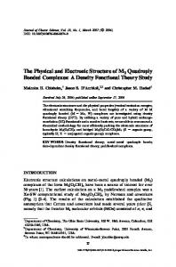
Figure Captions Fig.1 Plot of α(ω)/α(0) as a function of frequency ω for neon. The open and closed squares represent hydrodynamical and wavefunctional [38] results respectively. Fig.2 Plot of α(ω)/α(0) as a function of frequency ω for argon. The open and closed squares represent hydrodynamical and wavefunctional [38] results respectively. Fig.3 Static polarizability α(0) in the units of R03 of alkali metal clusters as a function of R0 . The filled squares represents the results of Kohn-Sham calculations [58]. Fig.4 Plot of γ(0) versus α(0) of alkali metal clusters. Fig.5 Plot of γ(ω; ω, −ω, ω) in the units of R03 as a function of frequency

ω for a metal cluster with 100 atoms.

28

α(ω)/α(0)

1.01

1.00 0.00

0.04

0.08

ω Fig. 1

α(ω)/α(0)

1.01

1.00 0.00

0.04

0.08

ω

α/R0

3

1.6

1.2

20

40

R0

Fig. 3

60

80

log(γ)

10

8

10

7

10

6

100

1000

log(α) Fig. 4

10000

12

γ(ω)

8

4

0 0.00

0.01

0.02

0.03

ω

0.04

0.05