Hydrodynamic tensor density functional theory with

THE JOURNAL OF CHEMICAL PHYSICS 126, 134101 共2007兲

Hydrodynamic tensor density functional theory with correct susceptibility Igor V. Ovchinnikov, Lizette A. Bartell, and Daniel Neuhausera兲 Department of Chemistry and Biochemistry, University of California at Los Angeles, Los Angeles, California, 90095-1569

共Received 9 June 2006; accepted 21 February 2007; published online 2 April 2007兲 In a previous work the authors developed a family of orbital-free tensor equations for the density functional theory 关J. Chem. Phys. 124, 024105 共2006兲兴. The theory is a combination of the coupled hydrodynamic moment equation hierarchy with a cumulant truncation of the one-body electron density matrix. A basic ingredient in the theory is how to truncate the series of equation of motion for the moments. In the original work the authors assumed that the cumulants vanish above a certain order 共N兲. Here the authors show how to modify this assumption to obtain the correct susceptibilities. This is done for N = 3, a level above the previous study. At the desired truncation level a few relevant terms are added, which, with the right combination of coefficients, lead to excellent agreement with the Kohn-Sham Lindhard susceptibilities for an uninteracting system. The approach is also powerful away from linear response, as demonstrated in a nonperturbative study of a jellium with a repulsive core, where excellent matching with Kohn-Sham simulations is obtained, while the Thomas-Fermi and von Weiszacker methods show significant deviations. In addition, time-dependent linear response studies at the new N = 3 level demonstrate the author’s previous assertion that as the order of the theory is increased new additional transverse sound modes appear mimicking the random phase approximation transverse dispersion region. © 2007 American Institute of Physics. 关DOI: 10.1063/1.2716667兴 I. INTRODUCTION

The development of new methods for quantum dynamics based upon hydrodynamic representations is very promising. In hydrodynamics the kinetics of the system is defined by a lesser number of variables than the number of variables required to define the complete one-particle density matrix 共which contains all the information on off-diagonal quantum coherence as in, e.g, the Kohn-Sham approach兲. For stationary studies the hydrodynamics approach is related to orbitalfree density functional theory.1–25 It is the reduced number of variables depicting the system that makes hydrodynamical theories applicable for numerical studies of relatively large systems. The simplest hydrodynamical approach is similar to the de Broglie–Bohm formulation of one-particle quantum mechanics.26–33 In this approximation the complete complexvalued one-particle density matrix is substituted by two real valued fields ␳ and ␾, which are combined in an order parameter ␺ = 冑␳ exp共i␸兲. The equations of motion are obtained by minimizing a Ginzburg-Landau-type functional on ␺. In addition the density matrix is assumed to possess longrange off-diagonal one-particle correlations. A more rigorous and asymptotically exact approach is an infinite hierarchy of coupled hydrodynamic moment 共CHM兲 equations.34–38 The moments come from a Taylor expansion of the one-particle density matrix with respect to the offdiagonal variable. To get a tractable system of equations the infinite hierarchy must be truncated. The most physically meaningful truncation is a cumulant expansion for the dena兲

Electronic mail: [email protected]

0021-9606/2007/126共13兲/134101/9/$23.00

sity matrix.34 Specifically, one decides on an order to terminate the method at; a low order will be less numerically demanding but less accurate than a higher one. Then, at that order, labeled N, the 共N + 1兲th order moment is expanded in terms of the previous set of moments, through the use of the cumulant expansion. The CHM theory and the accompanying cumulant truncation have been applied so far to systems where particle statistics does not play an important role. In Ref. 39 we have generalized the CHM theory and cumulant expansion to statistically degenerate fermions. The main point has been the modification of the unperturbed one-particle density matrix of a locally homogenous electron gas by using the cumulants. Since the approach uses successive tensors, we labeled it as hydrodynamic tensor density functional theory 共HTDFT兲. It turns out that the lowest level of truncation, N = 1, HTDFT corresponds to a de Brogilie–Bohm quantum hydrodynamics and in addition naturally incorporates the Thomas-Fermi40 kinetic energy term into the energy functional. At the next level, N = 2, HTDFT starts reproducing the spectrum of a homogenous Fermi liquid, i.e., it gets transverse excitations, rather than just classical plasmonic longitudinal excitations. The transverse sound mode mimics the elementary excitations’ density of states. A crucial feature of HTDFT is the value of the cumulant used at the truncation. In Ref. 39 we assumed that the 共N + 1兲th order cumulant is zero. It turns out, however, as we show here that this assumption leads to a wrong susceptibility for a homogenous electron gas, i.e., to a wrong linear response to a perturbation, even for a noninteracting system of electrons. We show here how to remedy this problem. This

126, 134101-1

© 2007 American Institute of Physics

Downloaded 22 Nov 2008 to 169.232.128.66. Redistribution subject to AIP license or copyright; see http://jcp.aip.org/jcp/copyright.jsp

134101-2

J. Chem. Phys. 126, 134101 共2007兲

Ovchinnikov, Bartell, and Neuhauser

is exemplified below for truncation at the N = 3 level, which is the first level where the method will yield different ground state results from the Thomas-Fermi approach. Specifically, the fourth order cumulant is written as a sum of terms involving the gradients of the previous moments. The coefficients of these terms are obtained by fitting to the exact susceptibility of a noninteracting set of electrons 共the Lindhard function兲. The balance of the paper is as follows. The general methodology is first developed in Sec. II. In Sec. III the derivation of a correct susceptibility is done. Section IV applies the methodology to a static nonperturbative numerical study of a jellium with a deep spherically symmetric hole, where we show that the agreement with Kohn-Sham results is excellent while the Thomas-Fermi and the von Weiszacker methods have significant errors. Section V is a linear response time-dependent study of the approach for N = 3 as a function of frequency and wave vector. This latter part is a direct continuation of our work in Ref. 39 for N = 2, and proves that there is an additional sound mode with respect to the N = 2 case, just as suggested in Ref. 39. Conclusions follow in Sec. VI. II. THE SYSTEM AND TENSOR-DFT FORMULATION A. Coupled hydrodynamic moment hierarchy

For completeness, we rederive the basic aspects of the theory 共see Ref. 39兲. We assume that the many electron system can be described by the one-particle density matrix ␳共1兲. The one-electron Hamiltonian governing this system h is, as usual, composed of kinetic terms and local potential terms. The one-particle density matrix is then expressed in terms of average and difference coordinates as

␳共1兲共R,s兲 = 具␺ˆ †共R − s/2兲␺ˆ 共R + s/2兲典.

共1兲

The time evolution of the one-particle density matrix is governed by the Heisenberg equation, i␳˙ = 关h , ␳兴, which in those coordinates takes the following form:

⳵ ˜ 共R + s/2兲 − ˜V共R − s/2兲兲␳共1兲 . i ␳共1兲共R,s兲 = Pˆ␣ pˆ␣␳共1兲 + 共V ⳵t

works we will aim to derive a form of Vxc which depends also on other moments in addition to ␳共R兲.兴 The particle kinetics in the system can be exactly described by the complete infinite set of hydrodynamic moments 共dynamic tensors兲,34–39 which are the derivatives of the one-particle density matrix with respect to the offdiagonal distance s at s = 0, ⌽l共N兲. . .l 共R兲 = pˆl1 . . . pˆlN␳共1兲兩共R,s兲兩s=0 . 1

共5兲

N

The particle and the current spatial densities are merely the first two tensors in the family, ⌽共0兲共R兲 = ␳共R兲,

⌽共1兲 i 共R兲 = Ji共R兲.

共6兲

By using Eq. 共2兲 one derives an infinite set of equations which connects the moments at different orders,

⳵ ␳ = − ⵜ ␣J ␣ , ⳵t

共7a兲

⳵ ˜ Ji = − ⵜ␣⌽i共2兲 ␣ − ␳ ⵜ iV , ⳵t

共7b兲

⳵ 共2兲 共3兲 ˜ ˜ ⌽ = − ⵜ␣⌽ik ␣ − J iⵜ kV − J kⵜ iV , ⳵t ik

共7c兲

⳵ 共3兲 共4兲 共2兲 ˜ 共2兲 ˜ 共2兲 ˜ ⌽ = − ⵜ␣⌽ikl ␣ − ⌽ik ⵜlV − ⌽il ⵜkV − ⌽lk ⵜiV ⳵t ikl + 41 ␳ⵜiⵜkⵜl˜V ,

共7d兲

.... This generic set of equations is correct for both fermions and bosons. For this set to be useful one should terminate it at some level. As usual, this termination is actually a method for factorizing a moment ⌽共N+1兲 at some N into moments ⌽k , k 艋 N. In addition, this truncation reflects the Fermi statistics of the particles. The order N at which one terminates controls the precision with which we treat the system.

共2兲 Here Pˆ␣ and pˆ␣ stand for the derivatives over the coordinates R␣ and s␣, Pˆ␣ = − i⳵/⳵R␣,

pˆ␣ = − i⳵/⳵s␣ ,

共3兲

and ˜V共R兲 is the effective potential, which also takes into account the two-body interactions, ˜V共R兲 =

冕

␳共R⬘兲 − ␳0共R⬘兲 3 ␦Exc d R⬘ − + Vext共R兲, 兩R − R⬘兩 ␦␳共R兲

共4兲

where ␳共R兲 = ␳共1兲共R , 0兲 is the spatial electron density, ␳0共R兲 is the positive nuclear charge density, Vext is any external potential, Exc is the exchange-correlation energy, and ␳0 is the nuclei density. There are a variety of functions Vxc ⬅ ␦Exc / ␦␳ in the literature 共see, e.g, Refs. 2–4兲. For us, however, the specific form of Vxc is not important. 关In future

B. Fermi factorization of higher order dynamic tensors

In Ref. 39 we proposed a factorization procedure for the lowest order dynamic tensors 共N = 2 , 3兲. Here we describe in detail how the factorization of the higher order dynamic tensors works in the Fermi case. The method proposed is based on the following general parametrization of the one-particle density matrix:

␳共1兲共R,s兲 = ␳ exp兵␾共R,s兲其f 0共␳,s兲,

␾共R,s兲 =

共8a兲

1

兺 ␾i共␣i兲 . . .i 共R兲共isi 兲共isi 兲 . . . 共isi 兲, ␣艌1 ␣!

f 0共␳,s兲 = 3

12

␣

1

2

sin共kFs兲 − 共kFs兲cos共kFs兲 , 共kFs兲3

␣

共8b兲

共8c兲

Downloaded 22 Nov 2008 to 169.232.128.66. Redistribution subject to AIP license or copyright; see http://jcp.aip.org/jcp/copyright.jsp

134101-3

J. Chem. Phys. 126, 134101 共2007兲

Hydrodynamic tensor density functional theory

kF = 共3␲2␳兲1/3 .

共8d兲

Here, f 0 is the normalized one-particle density matrix of a free fermion liquid with density ␳共R兲 and kF is the local 共density-dependent兲 Fermi wave vector. All the cumulants ␾共␣兲, are symmetric in all the indices because they are convolved with the symmetric tensors si1 . . . sin and all the ␾共␣兲 are real as the one-particle density matrix is hermitian. The same is true for the tensors ⌽共␣兲. The physical meaning of this parametrization is as follows. If ␾ ⬅ 0, then we end up with the Thomas-Fermi approximation of a locally homogeneous Fermi liquid. The ␾ function perturbs this steady liquid picture, and the tensors ␾␣’s and/or ⌽共␣兲’s determine different dynamic characteristics of the flowing electron liquid. The function f 0 assures the Fermi statistics of the particles at the one-particle level. For brevity we introduce below the tensors F

共␣兲

共␣兲

⬅ ⌽ /␳ ,

共9兲

instead of ⌽共␣兲. The tensors F共␣兲 and ␾共␣兲 are interrelated. The relations between F共␣兲’s and ␾共␣兲’s for the lowest order tensors are given below for the first four relations: F

共1兲

共1兲

=␾ ,

共10a兲

−1 e共4兲 ijkl = ␳ 具pi p j pk pl典ufs

= 3c4␦␦ijkl ⬅ c4共␦ij␦kl + ␦ik␦ jl + ␦il␦ jk兲,

共13兲

where the kinetic coefficients are defined as c2 = 51 kF2 ,

c4 =

1 4 35 kF .

共14兲

All the odd order e’s vanish. The general recipe for how to express F共N兲 in terms of ␾共␣兲’s is as follows. F共N兲 is the sum of all the different symmetrized 共in the sense discussed above兲 products of ␾␣ and e共␣兲 , ␣ 艋 N. An additional rule is that each term may include one 共and only one兲 e tensor. The relations inverse to Eqs. 共10兲 are F共1兲 − ␾共1兲 = 0,

共15a兲

F共2兲 − ␾共2兲 = F共1兲F共1兲 + e共2兲 ,

共15b兲

F共3兲 − ␾共3兲 = 3F共1兲F共2兲 − 2F共1兲F共1兲F共1兲 ,

共15c兲

F共4兲 − ␾共4兲 = 4F共1兲F共3兲 − 12F共1兲F共1兲F共2兲

F共2兲 = ␾共2兲 + ␾共1兲␾共1兲 + e共2兲 ,

共10b兲

+ 6F共1兲F共1兲F共1兲F共1兲 + 3F共2兲F共2兲 − 3e共2兲e共2兲

F共3兲 = ␾共3兲 + 3␾共1兲␾共2兲 + 3␾共1兲e共2兲 + ␾共1兲␾共1兲␾共1兲 ,

共10c兲

+ e共4兲 .

F共4兲 = ␾共4兲 + 4␾共1兲␾共3兲 + 3␾共2兲␾共2兲 + 6␾共1兲␾共1兲␾共2兲 + 6␾共2兲e共2兲 + 6␾共1兲␾共1兲e共2兲 + ␾共1兲␾共1兲␾共1兲␾共1兲 + e共4兲 , 共10d兲 etc. Here all terms are absolutely symmetric tensors of their indices so that there is no need to write down the indices explicitly; a bar denotes here a complete symmetrization, e.g., for a product of ai1. . .iK and bi1. . .iM , abi1. . .iK+M =

1 兺 ap共i1兲. . .p共iK兲bp共iK+1兲. . .p共iK+M兲 , 共K + M兲! p

where summation is assumed over all 共K + M兲! permutations of the indices and p denotes a permutation. The symmetrized multiplication is associative and it can be considered a multiplication on a ring of symmetric tensors 共note that in Ref. 39 a somewhat different symmetrization was used兲. Here is an explicit example of the symmetrized multiplication as follws: 共1兲 共2兲 共1兲 共1兲 共2兲 共1兲 共1兲 共2兲 ␾共1兲␾共1兲␾共2兲 ⬅ 61 共␾共1兲 i ␾ j ␾kl + ␾i ␾k ␾ jl + ␾i ␾l ␾ jk 共1兲 共2兲 共1兲 共1兲 共2兲 + ␾共1兲 k ␾l ␾ij + ␾ j ␾l ␾ik

+

共1兲 共2兲 ␾共1兲 j ␾k ␾il 兲. 共2兲

共4兲

In Eqs. 共10兲 the tensors e and e come from differentiating the function f 0, so that they have the physical meaning of averaging the particle momenta products over the unperturbed Fermi sea 共ufs兲: −1 e共2兲 ij = ␳ 具pi p j典ufs = c2␦ij ,

The inversion of the infinite set of relations 关Eq. 共10兲兴 is possible since an expression for any F共N兲 in terms of ␾共␣兲’s contains only ␾共␣兲 , ␣ 艋 N. This means that if one knows the expressions for the first N ␾共␣兲 tensors 关e.g, Eqs. 共15a兲–共15c兲 for N = 3兴 then by substituting all the lower order ␾共␣兲’s, ␣ 艋 N, in the relation for F共N+1兲 关Eq. 共10d兲兴 with corresponding expressions in terms of F共␣兲’s one gets the inverse relation for ␾共N+1兲 共Eq. 共15兲兲. The factorization for the tensor ⌽共N+1兲 is then simply given by the 共N + 1兲th equation in Eqs. 共15兲 The expression for the ⌽共N+1兲 tensor contains only kinetic tensors of order n 艋 N, as well as the 共N + 1兲th order cumulant. Once this cumulant is known the system of Eqs. 共8兲 closes and one arrives at the Nth order tensor DFT theory.

C. N = 3 hydrodynamic tensor DFT

At the N = 3 level the factorization of ⌽共4兲 is given by Eq. 共15d兲 with ␾共4兲 set to zero, or ⌽共4兲 = 4␳−1J⌽共3兲 − 12␳−2JJ⌽共2兲 + 6␳−3JJJJ + 3␳−1⌽共2兲⌽共2兲 − 3␳e共2兲e共2兲 + ␳e共4兲 + ␳␾共4兲 .

共11兲

共12兲

共15d兲

共16兲

In order to complete the theory we need to obtain ␾共4兲. For this, we study the static linear response of a homogeneous electron gas. In the ground state all the odd order ⌽共␣兲 tensors vanish 共a ground state has no currents as its wave function is real when there is no magnetic field and no degeneracy兲, so that the first three terms in Eq. 共16兲 would give only nonlinear contributions and can be neglected. As a

Downloaded 22 Nov 2008 to 169.232.128.66. Redistribution subject to AIP license or copyright; see http://jcp.aip.org/jcp/copyright.jsp

134101-4

J. Chem. Phys. 126, 134101 共2007兲

Ovchinnikov, Bartell, and Neuhauser

result, the required factorization for static studies simplifies as 共here we restore the indices兲 共4兲 2 −1 共2兲 共2兲 ⌽共4兲 ijkl = 3␳ ⌽ij ⌽kl + 3␳共c4共␳兲 − c2共␳兲兲␦ij␦kl + ␾ijkl .

共17兲

III. STATIC LINEAR RESPONSE OF HOMOGENEOUS FERMIONS AND ADJUSTMENT TO THE LINDHARD STRUCTURE FACTOR

The static properties of a homogeneous electron liquid are determined by the structure factor ␹共q兲. The structure factor is actually the static limit of the density-density correlation function ␹共q兲 = 兩具␳ˆ 共−q , −␻兲␳ˆ 共q , ␻兲典兩␻→i0. The physical meaning of ␹共q兲 is the ratio between the amplitude of the infinitesimal harmonic change in electron density ␳គ 共q兲 and that of the external potential vគ ext共q兲, which induces the change in the electron density,

␦vext共R兲 = vគ ext exp共iq · R兲 + c.c.,

共18a兲

␦␳共R兲 = ␳គ exp共iq · R兲 + c.c.,

共18b兲

␹共q兲 3 +¯ vគ ext + Cvគ ext ␳0

共18c兲

␳គ =

In the ground state of a homogeneous liquid the nonzero values at the N = 3 level are the density ␳0 and the second and 共4兲 the fourth order dynamic tensors ⌽共2兲 ij = ␳0c2共␳0兲␦ij and ⌽ijkl = ␳0c4共␳0兲␦¯· ␦ijkl. In a static linear response problem all the odd order kinetic tensors remain zero. Therefore, to study the static linear response of the system we let the values of ␳, ⌽共2兲, and ⌽共4兲 vary harmonically in space around their stationary values, vext = vគ exteiq·R + c.c.,

共19a兲

␳ = ␳0 + 共␳គ eiq·R + c.c.兲,

共19b兲

iq·R គ 共2兲 + c.c.兲, ⌽共2兲 ij = c2␳0␦ij + 共⌽ ij e

共19c兲

⌽共4兲 ijkl

= 3c4␳0␦ij␦kl +

iq·R 共⌽ គ 共4兲 ijkle

+ c.c.兲 +

ⵜi˜V = qi共i共˜v共q兲␳គ + vគ ext兲eiq·R + c.c.兲,

␳0␾共4兲 ijkl ,

共19d兲 共19e兲

where the underlined variables are the linear response coefficients, while ˜v共q兲 =

4␲ ⳵Vxc共␳兲 − 共␳0兲. q2 ⳵␳

共20兲

With the use of Eq. 共16兲 the infinitesimal deviation of ⌽共4兲 has the following form: 共4兲 គ 共2兲 ⌽ គ 共4兲 គ ␦ij␦kl + 6c2␦ij⌽ ijkl = 3D␳ kl + ␳0␾ijkl ,

where

共21兲

D=

冏

⳵共␳共c4 − c22兲兲 ⳵␳

冏

␳=␳0

− c22 = −

1 4 k . 15 F

Next we consider what terms can be in ␾共4兲. Our purpose is to make sure that the static response in the noninteracting case would resemble the Lindhard function 共static density response of free electrons兲. The terms added should include the derivative of the available quantities, i.e., the density and the stress tensor, so that they will be vanishing for uniform densities. Further, since ␾共4兲 is a fourth order tensor, it needs to be constructed from available tensors; the only ones available in the static limit are ⵜi, ␳, ⌽kl, and ␦ jl. It is easy to see by inspection that only the following local terms are available to first order in the perturbation and to lowest orders needed in ⵜi: 共2兲 ␳0␾共4兲 ijkl共R兲 = ⌳ⵜiⵜ jⵜkⵜl␳ − 6fⵜiⵜ j⌽kl − 6c2h␦ijⵜkⵜl␳ ,

共22兲 where ⌳, f, and h are dimensionless parameters. Even in linear response these terms can be augmented by terms involving further derivatives, e.g., terms involving a Laplacian of the components in Eq. 共22兲, 共i.e., q2 in Fourier space兲, but as orbital-free methods should be primarily geared towards the long-wavelength limit we do not consider here such higher order terms in q. The additional terms yield the following relation beគ 共2兲, and ⌽ គ 共4兲: tween the linear response coefficients ␳គ , ⌽ ⌽ គ 共4兲 គ 共2兲 គ ␦ij␦kl + ⌳␳គ qiq jqkql ijkl共q兲 = 6共c2␦ij + fqiq j兲⌽ kl + 3D␳ + 6c2h␳គ qiq j␦kl .

共23兲

Finally, the linearized equations read គ i共2兲 q ␣⌽ v␳គ + qi␳0vគ ext = 0, ␣ + qi␳0˜

共24a兲

and 2 គ k共2兲 គ 共2兲 3共c2␦ij + fqiq j兲共q␣⌽ ␣ 兲 + 3共c2 + fq 兲qi⌽ kl

+ 共3共D + c2␳0˜v + hc2q2兲␦ijqk + 共 41 ␳0˜v + ⌳q2 + 3hc2兲qiq jqk兲␳គ + 共3c2␦ijqk + 41 qiq jqk兲␳0vគ ext = 0,

共24b兲

where the index ␣ is summed over. The only preferential direction in the problem is the momentum vector q so that the dynamic tensor ⌽ គ 共2兲 can be decomposed into the following two form factors: គ 共0兲 + ⌽ គ 共2兲 ij = ␦ij⌽

qiq j 共1兲 ⌽ គ . q2

Upon substituting this resolution into the initial equations and equating independent spatial tensor components we arrive at three equations for ␳គ , ⌽ គ 共0兲, and ⌽ គ 共1兲,

Downloaded 22 Nov 2008 to 169.232.128.66. Redistribution subject to AIP license or copyright; see http://jcp.aip.org/jcp/copyright.jsp

134101-5

J. Chem. Phys. 126, 134101 共2007兲

Hydrodynamic tensor density functional theory

⌽ គ 共0兲 + ⌽ គ 共1兲 + ␳0˜v␳គ = − ␳0vគ ext ,

冉

共− ␳0vគ ext − ␳0˜v␳គ 兲 + 1 +

冉

+ −

冉

冊 冉 冊

kF2 + ␳0˜v + hq2 ␳គ = − ␳0vគ ext , 3

3f共− ␳0vគ ext − ␳0˜v␳គ 兲 + 3 +

冊

f 2 共0兲 q ⌽ គ c2

冊

f c2 1 + q2 ⌽ គ 共0兲 q2 c2

1 1 ␳0˜v + ⌳q2 + 3hc2 ␳គ = − ␳0vគ ext . 4 4

Upon solving these linear equations one gets

␳គ = − ␹␳0vគ ext ,

共25a兲

− ␹−1 = − ␹−1 v, 0 +˜

共25b兲

where −

1 + 20共2f − 1/12兲␩2 ␲2 ␹0 = , kF 1 − 24h␩2 − 80⌳␩4

共25c兲

and we introduced the following dimensionless momentum:

␩=

q . 2kF

Equation 共25b兲 is the definition of the structure factor renormalized with respect to two-body interactions. Therefore ␹0 should be the structure factor of noninteracting electrons. In order to adjust our theory to the realistic description of electrons one should compare ␹0 to the following Lindhard function:

冏 冏

1 1 − ␩2 1+␩ ␲2 − ␹Lind = + ln . 2 kF 4␩ 1−␩

共26兲

The freedom in choosing the parameters ⌳, f, and h allows us to fit our structure factor to the Lindhard function. The Lindhard function has the following properties:

␲ − ␹Lind = kF 2

冦

1 −2 3␩ , 1 − 31 ␩2 , 1 2,

␩→⬁ ␩→0 ␩ = 1.

冧

1 80 ,

f=

1 20 ,

and h = −

1 36 .

␳0共r兲 = ␳⬁ + ⌬␳共r兲,

冉

⌬␳共r兲 = − ␨␳⬁ 1 −

冊

r2 −r2/2r2 0, e 3r20

共29兲

where we took ␳⬁ = 0.01, ␨ = 0.9, and r0 = 3 and 2 共all in a.u.兲. The additional nonhomogeneous part of jellium density ⌬␳ integrates to zero so we avoid complications connected with an overall non-neutral system. Alternatively this system can be viewed as having constant jellium background density ␳⬁ but with an external Gaussian potential, Vb共r兲 = r20␨␳⬁

4␲ −r2/2r2 0, e 3

共30兲

which is related to ⌬␳共r兲 by the Poisson equation, 1 ⳵ 2⳵ r Vb共r兲 = 4␲⌬␳共r兲. r2 ⳵r ⳵r

共31兲

The Dirac exchange is used here, 共27兲 Vxc共R兲 =

In order for our function ␹0 to possess these properties we should choose ⌳=−

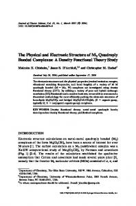
FIG. 1. The bare structure factors ␹0 on a scaled momentum scale q / 2kF for the 1 / 9 von Weiszacker approach, bare and adjusted ⌽共3兲 HTDFT theories, and the Lindhard function 共free-electron gas static density-density correlator兲. The ⌽共3兲 HTDFT is fitted to have the three properties of the Lindhard function given in Eq. 共27兲.

共28兲

A comparison between the resulting structure factor of the proposed theory with the Lindhard function and the structure factor provided by the 1 / 9 von Weiszacker theory is given in Fig. 1. IV. APPLICATION TO THE GROUND STATE PROBLEM

We applied the ⌽共3兲 theory to a ground state study of a nonperturbative nonhomogenous jellium. We chose a spherically symmetric infinite electron system in the following positive jellium background density profile:

共3␲2兲1/3 ␳共R兲1/3 . ␲

共32兲

No correlation energy was employed 共its contribution is very small; it will be included in future studies兲. The simulations were performed by adiabatical turning on the nonhomogeneous part of the jellium positive background density ⌬␳. Initially the electron and the jellium densities are homogeneous, ␳⬁. The odd order kinetic tensors Ji and ⌽共3兲 ijk are zero and the even order tensors are those of a homogeneous elec共2兲 共4兲 共4兲 tron liquid ⌽共2兲 ij = ␳⬁eij and ⌽ijkl = ␳⬁eijkl with the e tensors given in Eq. 共13兲. We then propagate the set of Eqs. 共7兲 while the jellium density gradually changes from homogenous to the final ␳0共r兲; this ensures that the system remains at the ground state for all times. We implemented the adiabatic density by setting

Downloaded 22 Nov 2008 to 169.232.128.66. Redistribution subject to AIP license or copyright; see http://jcp.aip.org/jcp/copyright.jsp

134101-6

J. Chem. Phys. 126, 134101 共2007兲

Ovchinnikov, Bartell, and Neuhauser

␳0共R,t兲 = 共1 − g共t兲兲␳0共R兲 + g共t兲␳⬁ , where g共t兲 is a smooth function rising from 0 to 1; we chose here, quite arbitrarily, g共t兲 =

1 , 1 + exp共共t0 − t/␶兲3兲

and used t0 = 3␶ . The width parameter ␶ was typically taken as 50 a.u.; this value was more than sufficient for adiabatic convergence. ␳0共R , t兲 is then used for the definition of the time-dependent potential 关Eq. 共4兲兴. The evolution of the system is then determined from the four first equations in Eq. 共7兲, with the ⌽共4兲 tensor given by Eqs. 共16兲 and 共22兲. The three dimensional equations were discretized and the derivative were evaluated by Fourier transforms, as was the Coulomb integral. Grid spacings of 1.6– 2 a.u. were sufficient to converge when the hole width parameter r0 was set at 2.0 or 3.0 a.u., respectively. A simple fixed step Runge-Kutta algorithm with dt = 0.2 a.u. was used to evolve the equations in time. We compared the results to Thomas-Fermi, von Weiszacker, and plane wave Kohn-Sham simulations. The latter were done by a standard plane wave code; interestingly, we found that the grid spacing needed to converge the KohnSham plane wave simulations had to be smaller by about 20% than those needed in the HFDFT code, so that they were about 1.3 and 1.6 a.u. for r0 = 2.0 and 3.0, respectively. The grids contained typically 共20兲3 points. Figure 2 shows that HTDFT gives essentially the same density as the Kohn-Sham approach, while the von Weiszacker and Thomas-Fermi results deviate significantly. Since the two-body interaction is treated the same in all four simulations, this proves that the hydrodynamic approach yields, even for this system which is shifted strongly away from uniformity, the same densities as the essentially exact description of the kinetic energy in the Kohn-Sham approach.

V. TIME-DEPENDENT LINEAR RESPONSE AND THE COLLECTIVE MODES 39

In our previous paper we studied the ground state of a homogenous electron gas at the N = 2 level, with the assumption that ␾共N+1兲 is zero. Here we extend the studies to N = 3, with ␾共4兲, as given by Eqs. 共22兲 and 共28兲. We derive the governing formulas in general, and arrive at analytical limits in the long-wavelength limit 共where ␾4 is not contributing兲, showing new kinds of excitations. In the ground state of a homogeneous liquid the nonzero values at the N = 3 level are the density ␳0 and the second and 共4兲 the fourth order dynamic tensors ⌽共2兲 ij = ␳0c2共␳0兲␦ij and ⌽ijkl = ␳0c4共␳0兲␦ij␦kl, respectively. To study the linear response of the system we let all the values in the problem vary harmonically around their stationary values,

␳ = ␳0 + 共␳គ e−i共␻t−q·R兲 + c.c.兲,

共33a兲

FIG. 2. The electron density profiles for a jellium model with background positive density 共lower solid line兲 given by Eq. 共29兲 with ␨ = 0.9 and r0 = 2 , 3 关共a兲 and 共b兲 graphs, respectively兴 for Thomas-Fermi, 1 / 9 von Weiszacker, ⌽共3兲 HTDFT, and the Kohn-Sham orbital based approaches. All quantities are in a.u.

Ji = Jគ ie−i共␻t−q·R兲 + c.c.,

共33b兲

−i共␻t−q·R兲 ⌽共2兲 គ 共2兲 + c.c.兲, ij = c2␳0␦ij + 共⌽ ij e

共33c兲

−i共␻t−q·R兲 គ 共3兲 + c.c., ⌽共3兲 ijk = ⌽ ijk e

共33d兲

ⵜi˜V = qi˜v共q兲共i␳គ e−i共␻t−q·R兲 + c.c.兲,

共33e兲

After linearizing Eqs. 共7兲 one gets

␻␳គ = q␣Jគ ␣ ,

共34a兲

␻Jគ i = q␣⌽ គ i共2兲 v共q兲␳គ , ␣ + ␳0qi˜

共34b兲

␻⌽ គ 共2兲 គ 共3兲 ij = q␣⌽ ij␣ ,

共34c兲

2 គ k共2兲 គ 共2兲 ␻⌽ គ 共3兲 ijk = 3共c2␦ij + fqiq j兲共q␣⌽ ␣ 兲 + 3共c2 + fq 兲qi⌽ jk

+ 共3共D + c2␳0˜v + hc2q2兲␦ijqk + 共 41 ␳0˜v + ⌳q2 + 3hc2兲qiq jqk兲␳គ ,

共34d兲

where the linearized variation of ⌽共4兲 is taken from Eq. 共23兲, and ␣ is again summed over. This is a system of linear homogeneous equations, and to find its solutions we have to diagonalize it. All the variables in Eqs. 共34兲 could be expressed in terms of ␳គ and ⌽ គ 共2兲 ij . Therefore, we can consider the equations on ⌽ គ 共2兲 and ␳គ only without losing any solutions. In matrix form these equations read

Downloaded 22 Nov 2008 to 169.232.128.66. Redistribution subject to AIP license or copyright; see http://jcp.aip.org/jcp/copyright.jsp

134101-7

J. Chem. Phys. 126, 134101 共2007兲

Hydrodynamic tensor density functional theory

␻2 ␳គ = Tr共⌽ គ 共2兲Q兲 + ␳0˜v共q兲␳គ , q2

共35a兲

␻2 共2兲 ⌽ គ = 共c2 + fq2兲共⌽ គ 共2兲 + 2兵⌽ គ 共2兲,Q其兲 q2 共2兲

គ Q兲 + 共c2I + fq Q兲Tr共⌽ 2

+ 共IZ共q兲 + QZ⬘共q兲兲␳គ ,

共35b兲

⌽ គ 共2兲 = ␣Q + ␤共I − Q兲,

共40兲

which leads, upon insertion into Eqs. 共35兲, to the following equations for ␣, ␤, and ␳គ :

␻2 ␣ = 6共c2 + fq2兲␣ + 共Z共q兲 + 共Z⬘共q兲兲␳គ . q2

共41a兲

␻2 ␤ = c2␣ + 共c2 + fq2兲␤ + Z共q兲␳គ , q2

共41b兲

␻2 ␳គ = ␣ + ␳0˜v共q兲␳គ . q2

共41c兲

where Z共q兲 = D + c2␳0˜v + hc2q2 , Z⬘共q兲 = 2Z + 41 ␳0˜v共q兲q2 + ⌳q4 + 3hc2q2 , and Tr means a matrix trace, Iij ⬅ ␦ij is the 3 ⫻ 3 unity matrix, Qij = qiq j / q2, curly brackets denote an anticommutator, and capital bold face letters refer here to matrices. Without loss of generality we can always assume that the wave vector q is directed along the x axis 共q = 共q , 0 , 0兲T兲, so that

冢 冣 1 0 0

共36兲

Q= 0 0 0 . 0 0 0

There are several solutions for these equations. The first three solutions are decoupled from the density fluctuations so that ␳គ = 0 for all of them. They are

冢 冣冢 冣 0 1 0

0 0 1

⌽ គ 共2兲 = 1 0 0 , 0 0 0

0 0 0 , 1 0 0

共37a兲

共37b兲

and

冢 冣 0 0 0

⌽ គ

共2兲

共38a兲

= 0 0 1 , 0 1 0

with a dispersion of

␻2 = 1/5kF2 q2 .

共38b兲

The first two solutions 关Eq. 共37a兲兴 correspond to transverse sound as the current is given as

冢冣 冢冣 0

␻共q兲Ji =

q j⌽ គ 共2兲 ij

= q , 0

0

0 . q

冢

6

0

3

1

1

1

a共q兲 0 a共q兲

冣冢 冣 冢 冣 ␣ ␤ = ␻ ⬘2 ␳គ ⬘

␣ ␤ , ␳គ ⬘

共42兲

where a共q兲 = 4␲␳0 / 共q2c2兲, ␻⬘2 = ␻2 / 共q2c2兲, ␳គ = 4␲␳0␳គ / q2, and a共q兲 Ⰷ 1. Dropping the terms of order a共q兲−1 and smaller, the three eigenvalues and corresponding eigenvectors are

␻2 = 51 kF2 q2,

共␣, ␤, ␳គ ⬘兲 = 共1,2/3,− 1兲;

共43a兲

␻2 = 53 kF2 q2,

共␣, ␤, ␳គ ⬘兲 = 共1,0,− 1兲;

共43b兲

␻2 = ␻2P + 53 kF2 q2,

which corresponds to the following dispersion relation:

␻2 = 3/5kF2 q2 ,

This set of equations has complicated solutions, which, however, could be simplified in low-wavelength limit. In this limit, we can leave only the leading terms in q; in the effective potential it is the divergent Fourier components of the Coulomb potential. In the long-wavelength limit the system of equations has the following form:

共␣, ␤, ␳គ ⬘兲 = 共0,0,1兲,

共43c兲

where ␻2P = 4␲␳0 is the plasmon frequency. Note that the first two of the three modes 关Eq. 共43a兲 and 共43b兲兴 have the same eigenvalues as the transverse modes in Eqs. 共37b兲 and 共38b兲. The total spectrum given by N = 3 HTDFT for elementary excitations in the homogeneous electron gas is given in Fig. 3. The spectrum found differs from that of the N = 2 approach by an additional sound mode with velocity 冑3 / 5kF and by shifting the previous sound modes from 冑3 / 5kF to 冑1 / 5kF. This result confirms the conjecture made in Ref. 39, that with increasing N new sound modes should appear, and that they will gradually cover the entire continuous random phase approximation 共RPA兲 density of states in the Fermi liquid.

共39兲

Note, however, that the velocity of this transverse sound mode is different from the one found for the same mode within the N = 2 theory.39 The third solution in Eq. 共38兲 is a new sound mode. This mode involves neither density nor current fluctuations and corresponds to transverse quadrupole fluctuations of the Fermi sea. The next three solutions are found by representing the tensor ⌽共2兲 in terms of the remaining diagonal tensors 共I and Q兲,

VI. CONCLUSIONS

In conclusion, we have shown that HTDFT can also be used for time-independent studies. We have supplanted our previous conjecture where we assumed that the terms in the equation of motion hierarchy should be terminated with the next relevant cumulant 关i.e., ␾共N+1兲兴 being zero; instead, we now derived ␾共N+1兲 from fitting the linear response to a HEG. The resulting set of equations 关given at the N = 3 level by Eqs. 共22兲, 共7兲, and 共16兲兴 is closed and can be propagated forward in time.

Downloaded 22 Nov 2008 to 169.232.128.66. Redistribution subject to AIP license or copyright; see http://jcp.aip.org/jcp/copyright.jsp

134101-8

J. Chem. Phys. 126, 134101 共2007兲

Ovchinnikov, Bartell, and Neuhauser

FIG. 3. The elementary excitation spectrum provided by quantum hydrodynamics, HTDFT ⌽共2兲, and HTDFT ⌽共3兲 theories. QH gives only a plasmon mode. HTDFT also gives transverse sound modes which mimic the RPA elementary excitations in Fermi liquid. ⌽共3兲 HTDFT gives additional sound modes with respect to ⌽共2兲 HTDFT confirming the conjecture made in Ref. 39 that when increasing the order of HTDFT new sound modes should appear, and they will gradually cover the entire continuous RPA density of states of Fermi liquid.

The linear response in the static limit is fitted to the Lindhard function homogeneous electron gas 共HEG兲 for both short, intermediate, and long wavelengths 共for comparison, the 1 / 9 in the von Weiszacker approach is obtained to fit long wavelengths, while a fit to long wavelengths would have required replacing the 1 / 9 by 1 in the von Weiszacker theory兲. We have then applied HTDFT away from equilibrium, for a case of a jellium density with a deep hole in the middle, and have shown excellent agreement with the KohnSham results, in a case where more approximate theories such as Thomas-Fermi and von Weiszacker fail; this is directly due to the fact that their structure factor do not follow the Lindhard function except at low wavelengths. The last part of the paper dealt with time-dependent linear response studies at the present level N = 3. The analytical studies have confirmed our previous assertion that as the level of the theory increases more and more transverse excitations are found. A new excitation at the N = 3 level couples neither to the current nor to the density. All excitations, including the new ones, lie within the RPA density of stats of elementary excitations in a Fermi liquid. Future works will study the applicability of the approach to covalent chemical systems, where the directionality of the tensors should enable a correct description even at a low N, possibly as low as N = 3. Further, dynamic susceptibilities will be studied so that further terms, depending on J, ⌽共3兲, etc., will be included in the terminating cumulant 关␾4 here, ␾共N+1兲 in general兴 so that the theory will be valid over a wide range of frequencies and wave vectors. Of course, it will be very interesting and challenging for the theory to get the correct material-specific band gaps, since in many covalent systems the band gap is extremely material dependent. Therefore, the earliest efforts in the theory will be towards quasifree metallic systems, such as metallic dots and their interaction. The basic formalism developed here and in forthcoming work will be useful in developing applications to

dynamical problems which straddle the transition between molecular system and nanostructures, at least for metallic systems. Another direction is the application to magnetic phenomena. We have separately shown that the HTDFT approach is naturally appropriate to describe magnetic vortices and the transition between different ferromagnetic phases. This will be presented in a separate publication. We note that other applications to fermionic systems can also be envisioned. For example, by replacing the zeroth order HEG density matrix with a temperature-dependent density matrix and fitting the coefficients of the derivative terms in the cumulant to a temperature dependent Lindhard expression, we will get a temperature-dependent HTDFT theory which can be applied to plasmas and to studies of narrow conduction bands. Similarly, applications to nuclear systems can also be envisioned. Other future improvements will include better methods to solve the time-dependent HTDFT equations. One approach will be to include external electric fields that will have dipole and quadruple 共or higher兲 components that will be time dependent. The electric fields will be chosen, at each time instant, to remove energy from the system 关i.e., to reduce the trace of ⌽共2兲 plus the total potential兴. ACKNOWLEDGMENTS

The authors thank Roi Baer for doing the Kohn-Sham studies, help analyzing the linear response, and for extensive discussions. Helpful comments by Emily Carter are greatly appreciated. This work was supported by the NSF and PRF. 1

R. G. Parr and W. Yang, Density-Functional Theory of Atoms and Molecules 共Oxford University Press, New York, 1989兲; R. M. Dreizler and E. K. U. Gross, Density Functional Theory: An Approach to the Quantum Many-Body Problem 共Springer-Verlag, Berlin, 1990兲. 2 Y. A. Wang, N. Govind, and E. A. Carter, Phys. Rev. B 60, 16350 共1999兲. 3 Y. A. Wang, N. Govind, and E. A. Carter, Phys. Rev. B 58, 13465 共1998兲. 4 L. B. Zhou, V. L. Ligneres, and E. A. Carter, J. Chem. Phys. 122, 044103 共2005兲. 5 P. Garcia Gonzalez, J. E. Alvarellos, and E. Chacon, Phys. Rev. A 54, 1897 1996; , Phys. Rev. B 53, 9509 共1996兲; Phys. Rev. B 57, 4857 共1998兲. 6 E. Smargiassi and P. A. Madden, Phys. Rev. B 49, 5220 共1994兲; 51, 117 共1995兲. 7 Q. Wang, M. D. Glossman, M. P. Iniguez, and J. A. Alonso, Philos. Mag. B 69, 1045 共1993兲. 8 S. C. Watson and P. A. Madden, Phys. Chem. Commun. 1, 1 共1998兲; S. C. Watson and E. A. Carter, Comput. Phys. Commun. 128, 67 共2000兲. 9 N. Govind, J. Wang, and H. Guo, Phys. Rev. B 50, 11175 共1994兲; N. Govind, J. L. Mozos, and H. Guo, ibid. 51, 7101 共1995兲. 10 D. Nehete, V. Shah, and D. G. Kanhere, Phys. Rev. B 53, 2126 共1996兲. 11 A. Aguado, J. M. Lopez, J. A. Alonso, and M. J. Stott, J. Chem. Phys. 111, 6026 共1999兲; J. Phys. Chem. B 105, 2386 共2001兲. 12 A. E. Depristo and J. D. Kress, Phys. Rev. A 35, 438 共1987兲. 13 L. W. Wang and M. P. Teter, Phys. Rev. B 45, 13196 共1992兲. 14 M. Brack, B. K. Jennings, and Y. H. Chu, Phys. Lett. B 65, 1 共1976兲. 15 T. J. Frankcombe, G. J. Kroes, N. I. Choly, and E. Kaxiras, J. Phys. Chem. B 109, 16554 共2005兲. 16 E. Sim, J. Larkin, K. Burke, and C. W. Bock, J. Chem. Phys. 118, 8140 共2003兲. 17 P. W. Ayers, J. Math. Phys. 46, 062107 共2005兲. 18 G. K. L. Chan, A. J. Cohen, and N. C. Handy, J. Chem. Phys. 114, 631 共2001兲. 19 N. Choly and E. Kaxiras, Phys. Rev. B 67, 155101 共2003兲; , Solid State

Downloaded 22 Nov 2008 to 169.232.128.66. Redistribution subject to AIP license or copyright; see http://jcp.aip.org/jcp/copyright.jsp

134101-9

Commun. 121, 281 共2002兲. M. D. Glossman, A. Rubio, L. C. Balbas, and J. A. Alonso, Int. J. Quantum Chem. 45, 333 共1993兲; 49, 171 共1994兲. 21 E. K. U. Gross and R. M. Dreizler, Phys. Rev. A 20, 1798 共1979兲. 22 H. Lee, C. T. Lee, and R. G. Parr, Phys. Rev. A 44, 768 共1991兲. 23 G. I. Plindov and S. K. Pogrebnya, Chem. Phys. Lett. 143, 535 共1988兲. 24 W. T. Yang, Phys. Rev. A 34, 4575 共1986兲. 25 B. Weiner and S. B. Trickey, Adv. Quantum Chem. 35, 217 共1999兲. 26 E. Madelung, Z. Phys. 40, 322 共1926兲; L. de Broglie, Acad. Sci., Paris, C. R. 183, 447 共1926兲; 184, 273 共1927兲; D. Bohm, Phys. Rev. 85, 166 共1952兲; 85, 180 共1952兲. 27 A. K. Roy and S. I. Chu, Phys. Rev. A 65, 043402 共2002兲; A. K. Roy, N. Gupta, and B. M. Deb, ibid. 65, 012109 共2002兲; B. M. Deb and P. K. Chattaraj, ibid. 39, 1696 共1989兲. 28 C. L. Lopreore and R. E. Wyatt, Phys. Rev. Lett. 82, 5190 共1999兲. 29 R. E. Wyatt, Chem. Phys. Lett. 313, 189 共1999兲; R. E. Wyatt and E. R. Bittner, J. Chem. Phys. 113, 8898 共2000兲; C. J. Trahan, R. E. Wyatt, and B. Poirier, ibid. 122, 164104 共2005兲. 30 J. C. Burant and J. C. Tully, J. Chem. Phys. 112, 6097 共2000兲. 20

J. Chem. Phys. 126, 134101 共2007兲

Hydrodynamic tensor density functional theory

B. K. Day, A. Askar, and H. A. Rabitz, J. Chem. Phys. 109, 8770 共1998兲; F. S. Mayor, A. Askar, and H. A. Rabitz, ibid. 111, 2423 共1999兲. 32 D. Nerukh and J. H. Frederick, Chem. Phys. Lett. 332, 145 共2000兲. 33 S. W. Derrickson, E. R. Bittner, and B. K. Kendrick, J. Chem. Phys. 123, 054107 共2005兲. 34 E. R. Bittner, J. B. Maddox, and I. Burghardt, Int. J. Quantum Chem. 89, 313 共2002兲; J. B. Maddox and E. R. Bittner, J. Phys. Chem. B 106, 7981 共2002兲. 35 I. Burghardt, J. Chem. Phys. 122, 094103 共2005兲. 36 M. Ploszajczak and M. J. Rhoades-Brown, Phys. Rev. Lett. 55, 147 共1985兲; Phys. Rev. D 33, 3686 共1986兲. 37 J. V. Lill, M. I. Haftel, and G. H. Herling, Phys. Rev. A 39, 5832 共1989兲; J. Chem. Phys. 90, 4940 共1989兲. 38 L. M. Johansen, Phys. Rev. Lett. 80, 5461 共1998兲. 39 I. V. Ovchinnikov and D. Neuhauser, J. Chem. Phys. 124, 024105 共2006兲. 40 L. H. Thomas, Proc. Cambridge Philos. Soc. 23, 542 共1927兲; E. Fermi, Rend. Accad. Naz. Lincei 6, 602 共1927兲; , Z. Phys. 48, 73 共1928兲. 31

Downloaded 22 Nov 2008 to 169.232.128.66. Redistribution subject to AIP license or copyright; see http://jcp.aip.org/jcp/copyright.jsp