Hyperbolic Harmonic Mapping for Constrained Brain Surface Registration Rui Shi1 , Wei Zeng2 , Zhengyu Su1 , Hanna Damasio3 , Zhonglin Lu4 , Yalin Wang5 , Shing-Tung Yau6 , and Xianfeng Gu1 1
Department of Computer Science@Stony Brook University School of Computing & Information Sciences@Florida International University 3 School of Computing, Informatics, and Decision Systems Engineering@Arizona State University 4 Neuroscience@University of Southern California 5 Department of Psychology@Ohio State University 6 Mathematics Department@Harvard University {
[email protected];
[email protected];
[email protected];
[email protected];
[email protected];
[email protected];yau@math. harvard.edu;
[email protected]} 2
Abstract
search: similarity and correspondence. Examples of similarity research include 3D face recognition [5], shape retrieval [6], etc. Among various correspondence research, automatic computation of surface correspondence regulated by certain geometric or functional constraints is an important research field in computer vision and medical imaging. For example, in human brain mapping research, since cytoarchitectural and functional parcellation of the cortex is intimately related the folding of the cortex, it is important to ensure the alignment of the major anatomic features, such as sucal landmarks. Among various rigid and non-rigid surface registration approaches (e.g. [3, 5, 16]), harmonic map is one of the most broadly applied methods [27, 32]. The advantages of harmonic map computation are: (1) it is physically natural and can be computed efficiently; (2) it measures the elastic energy of the deformation so it has clear physical interpretation; (3) for a planar convex domain, it is diffeomorphism; (4) it can be computed by solving an elliptic partial differential equation so its computation is numerically stable; (5) it continuously depends on the boundary condition so it can be controlled by adjusted boundary conditions. In computer vision and medical imaging fields, surface harmonic map has been used to compute spherical conformal mapping [12], image registration [13], high resolution tracking of non-rigid motion [27], non-rigid surface registration, etc. However, the current state-of-the-art surface harmonic map research has some limitations. For example, it usually only works with genus zero surfaces but does not work with general topology surfaces. It is hard to add landmark
Automatic computation of surface correspondence via harmonic map is an active research field in computer vision, computer graphics and computational geometry. It may help document and understand physical and biological phenomena and also has broad applications in biometrics, medical imaging and motion capture. Although numerous studies have been devoted to harmonic map research, limited progress has been made to compute a diffeomorphic harmonic map on general topology surfaces with landmark constraints. This work conquer this problem by changing the Riemannian metric on the target surface to a hyperbolic metric, so that the harmonic mapping is guaranteed to be a diffeomorphism under landmark constraints. The computational algorithms are based on the Ricci flow method and the method is general and robust. We apply our algorithm to study constrained human brain surface registration problem. Experimental results demonstrate that, by changing the Riemannian metric, the registrations are always diffeomorphic, and achieve relative high performance when evaluated with some popular cortical surface registration evaluation standards.
1. Introduction Analysis and understanding of shapes is one of the most fundamental tasks in our interaction with the surrounding world. There are two major problems in shape analysis re1
curve information. A harmonic map combined with landmark matching conditions usually does not guarantee diffeomorphism. All these problems become obstacles to apply harmonic map to solve general non-rigid surface matching problems. In contrast, in current work, we slice along the landmark curves on general surfaces and assign a unique hyperbolic metric on the template surface, such that all the boundaries become geodesics. Then by establishing harmonic mappings, the obtained surface correspondences are guaranteed to be diffeomorphic. In this paper, we apply the proposed method to study human brain cortical surface registration problem. Early research [11, 24] has demonstrated that surface-based approaches may offer advantages as a method to register brain images. The cortical surface registration may help identify early disease imaging biomarkers, develop new treatments and monitor their effectiveness, as well as lessen the time and cost of clinical trials. In summary, the main contributions of the current work are as follows: 1. Introduce a novel algorithm to compute harmonic mappings on hyperbolic metric using nonlinear heat diffusion method and Ricci flow. 2. Develop a novel brain registration method based on hyperbolic harmonic maps. The new method overcomes the shortcomings of the conventional methods, such that the registration is guaranteed to be diffeomorphic. 3. Introduce a novel general methodology to achieve special goals in geometric processing by changing the surface Riemannian metrics.
all, finding diffeomorphic mappings between brain surfaces is an important but difficult problem. In most cases, extra regulations, such as inverse consistency [23], have to be enforced to ensure a diffeomorphism. Since the proposed work offers a harmonic map based scheme for diffeomorphisms which guarantees a perfect landmark curve registration via enforced boundary matching, the novelty of the proposed work is that it facilitates diffeomorphic mapping between general surfaces with delineated landmark curves.
3. Theoretic Background This section briefly covers the most relevant concepts and theorems of harmonic maps [21] and surface Ricci flow [31]. Ricci Flow Suppose (S, g) is a compact surface embedded in R3 , g is the induced Euclidean metric. Definition 3.1 (Surface Ricci Flow) The normalized surface Ricci flow is defined as ( ) dg(t) 2πχ(S) =2 − K(t) g(t) dt A(0) where χ(S) is the Euler characteristic number of S, A(0) is the total area of the surface at time 0, K(t) is the Gaussian curvature induced by g(t). Theorem 3.2 (Hamilton) If χ(S) < 0, then the solution to the normalized Ricci flow equation exists for all t > 0 and converges to a metric with constant curvature 2πχ(S) A(0) .
2. Previous Works
By running Ricci flow, a hyperbolic metric of the surface can be obtained, which induces −1 Gaussian curvature everywhere.
In computer vision and medical imaging research, surface conformal parameterization with the Euclidean metric have been extensively studied [1, 22, 31, 30, 4, 28]. Wang et al. [26] studied brain morphology with Teichm¨uller space coordinates where the hyperbolic conformal mapping was computed with the Yamabe flow method. Zeng [31] proposed a general surface registration method via the Klein model in the hyperbolic geometry where they used the inversive distance curvature flow method to compute the hyperbolic conformal mapping. Various surface registration methods were proposed in computer vision field [7, 19, 16, 17]. To register brain cortical surfaces, a common approach is to compute a range of intermediate mappings to some canonical parameter space [24, 11, 29]. A flow, computed in the parameter space of the two surfaces, then induces a correspondence field in 3D [8]. This flow can be constrained using anatomical landmark points or curves [2, 14, 20, 33], by sub-regions of interest [15], by using currents to represent anatomical variation [10], or by metamorphoses [25]. There are also various ways to optimize surface registrations [4, 18, 23]. Over-
Hyperbolic Plane The Poincar´e’s disk model for the hyperbolic plane H2 is the unit disk on the complex plane {z ∈ C| |z| < 1} with Riemannian metric (1 − z z¯)−2 dzd¯ z. The geodesics (hyperbolic lines) are circular arcs perpendicular to the unit circle. The hyperbolic rigid motions are M¨obius transformations ϕ : z → eiθ (z − z0 )/(1 − z¯0 z). The axis of ϕ is the hyperbolic line through its fixed points: z1 = limn→∞ ϕn (z), z2 = limn→∞ ϕ−n (z). Given two non-intersecting hyperbolic lines γ1 and γ2 , there exists a unique hyperbolic line τ orthogonal to both of them, and gives the shortest path connecting them. For each γk , there is a unique reflection ϕk whose axis is γk , then the axis of ϕ2 ◦ ϕ−1 1 is τ . Another hyperbolic plane model is the Klein’s disk model, where the hyperbolic lines coincide with Euclidean lines. The conversion from Poincar´e’s disk model to Klein disk model is given by z → 2z/(1 + z z¯). 2
Fundamental Group and Fuchs Group Let S be a surface, q ∈ S is a base point. Consider all the loops through q. Two loops are homotopic, if one can deform to the other without leaving S. The product of two loops is the concatenation of them. All the homotopy classes of loops form the fundamental group (homotopy group), denoted as π1 (S, q). Furthermore, all the homotopic classes of paths on the ˜ surface starting from p form a simply connected surface S, the projection map p : S˜ → S maps each path to its end point, the projection map is a local homeomorphism. The ˜ p) is called the universal covering space of S. pair (S, Suppose S is with a hyperbolic metric, then its universal covering space S˜ can be isometrically embedded onto the hyperbolic plane H2 . A Fuchsian transformation ϕ is a M¨obius transformation, that preserves the projection ϕ ◦ p = p. All Fuchsian transformations form the Fuchs group, F uchs(S), which is isomorphic to the fundamental group π1 (S, q). Choose a base point q˜ ∈ H2 , p(˜ q ) = q. A path γ˜ ∈ H2 connecting q˜ and ϕ(˜ q ), then the projection p(˜ γ ) is a loop on the base surface S. The axis of ϕ is the unique geodesic in the homotopy class of p(˜ γ ).
g1 = σ(z)dzd¯ z and g2 = ρ(w)dwdw. ¯ Then the mapping has local representation w = f (z) or denoted as w(z). Definition 3.3 (Harmonic Map) The harmonic energy of the mapping is defined as ∫ E(f ) = ρ(z)(|wz |2 + |wz¯|2 )dxdy S
If f is a critical point of the harmonic energy, then f is called a harmonic map. The necessary condition for f to be a harmonic map is the Euler-Lagrange equation wzz¯ + ρρw wz wz¯ ≡ 0. The following theorem lays down the theoretic foundation of our proposed method. Theorem 3.4 [21] Suppose f : (S1 , g1 ) → (S2 , g2 ) is a degree one harmonic map, furthermore the Riemannian metric on S2 induces negative Gauss curvature, then for each homotopy class, the harmonic map is unique and diffeomorphic.
4. Algorithms In this section we first explain our registration algorithm pipeline as illustrated in Alg. 1 and Fig. 1:
Hyperbolic Pants Decomposition A pair of pants is a genus zero surface with 3 boundaries. Any surfaces S with complicated topology can be decompose to |χ(S)| pairs of pants. If S has a hyperbolic metric, then all the cutting loops can be chosen to be geodesics, as shown in Fig.2 (a) and (b). Furthermore, each pair of hyperbolic pants can be further decomposed. Assume the pair of pants have three geodesic boundaries {γi , γj , γk }. Let {τi , τj , τk } be the shortest geodesic paths connecting each pair of them. The shortest paths divide the surface to two identical hyperbolic hexagons with right inner angles. when mapped to the Klein’s model, the hyperbolic hexagons coincide with convex Euclidean hexagons.
Algorithm 1 Brain Surface Registration Algorithm Pipeline. 1. Slice the cortical surface along the land marks. 2. Compute the hyperbolic metric using Ricci flow. 3. Hyperbolic pants decomposition, isometrically embed them to Klein model. 4. Compute harmonic maps using Euclidean metrics between corresponding pairs of pants, with consistent boundary constraints. 5. Use nonlinear heat diffusion to improve the mapping to a global harmonic map on Poincar´e disk model.
Harmonic Map Suppose S is a closed oriented surface with a Riemannian metric g, by running surface Ricci flow, one can obtain a Riemannian metric with constant curvature +1, 0, −1 everywhere. The universal covering space of the surface can be isometrically embedded onto the sphere C ∪ {∞}, the Euclidean plane C or the hyperbolic plane H2 . This process is called the uniformization of the surface. Based on the uniformization, one can construct an atlas, such that on each chart {z}, the original Riemannian metric g = σ(z)dzd¯ z , which is called the isothermal parameters of the surface. An atlas consisting of isothermal parameter charts is called an conformal structure. It is convenient to use complex differential operator ∂z = 1/2(∂x + i∂y ) and ∂z¯ = 1/2(∂x − i∂y ). Given a mapping f : (S1 , g1 ) → (S2 , g2 ), z and w are local isothermal parameters on S1 and S2 respectively.
1. Preprocessing The cortical surfaces are reconstructed from MRI images and represented as triangular meshes. The sucal landmarks are manually labeled on the edges of the meshes. Then we slice the meshes along the landmark curves, to form topological multiple connected annuli. 2. Discrete Hyperbolic Ricci Flow Because the Euler characteristic number of the cortical surfaces are negative, they admit hyperbolic metrics. We treat each triangle as a hyperbolic triangle and set the target Gauss curvatures for each interior vertex to be zeros, and the target geodesic curvature for each boundary vertex to be zeros as well. Then compute the hyperbolic metrics of the brain meshes using discrete hyperbolic Ricci flow method [31]. Algorithm 2 describes the details. 3
boundary loop, compute its corresponding M¨obius transfor−∞ mation, ϕγi γj , and its fixed points ϕ+∞ γi γj (0) and ϕγi γj (0). The hyperbolic line through the fixed points is the axis of the ϕγi γj , which is the geodesic in [γi γj ]. Slice the mesh along the geodesic, and repeat the process on each connected components, until all the connected components are pairs of pants. Fig 2 (a) shows how to decompose a closed surface into pant surface (b). (c) and (d) show an example of the pant decomposition process on open boundary surfaces. Alg. 3 gives the computational steps.
Figure 1. Algorithm Pipeline (suppose we have 2 brain surface M and N as input): (a). The input brain models M and N , with landmarks been cut open as boundaries. (b). Hyperbolic embedding of the M and N on Poincar´e disk. (c). Decompose M and N into multiple pants by cut the landmarks into boundaries, and each pant further decomposed to 2 hyperbolic hexagons. (d). Hyperbolic hexagons on Poincar´e disk become convex hexagons under Klein model, then a one-to-one map between the correspondent parts of M and N can be obtained. Then we can apply our hyperbolic heat diffusion algorithm to get a global harmonic diffeomorphism. (e). Color coded registration result of M and N .
Figure 2. Hyperbolic pants decomposition. (a) shows an arbitrary closed surface can be decomposed into multiple pant surfaces. (b) shows a pant surface. For open boundaries surfaces, we cut along γ ′ which is the geodesic loop of homotopy class of [γ0 · γ1 ] ((c) and (d)). Repeat it until all pants are decomposed.
Algorithm 2 Discrete Hyperbolic Ricci Flow. Input: Surface M . Output: The hyperbolic metric U of M . 1. Assign a circle at vertex vi with radius ri ; For each edge [vi , vj ], two circles intersect at an angle ϕij , called edge weight. 2. The edge length lij of [vi , vj ] is determined by the hyperbolic cosine law: coshlij = coshri coshrj + sinhri sinhrj cosϕij 3. The angle θijk , related to each corner , is determined by the current edge lengths with the inverse hyperbolic cosine law. 4. Compute the discrete Gaussian curvature Ki of each vertex vi : { ∑ 2π − fijk ∈F θijk , interior vertex ∑ (1) Ki = π − fijk ∈F θijk , boundary vertex
Algorithm 3 Hyperbolic Pants Decomposition. Input: Topological sphere M with B boundaries. Output: Pants decomposition of M . 1. Put all boundaries γi of M into a queue Q. 2. If Q has < 3 boundaries, end; else goto Step 2. 3. Compute a geodesic loop γ ′ homotopic to γi · γj 4. γ ′ , γi and γj bound a pants patch, remove this pants patch from M . Remove γi and γj from Q. Put γ ′ into Q. Go to Step 1.
4. Constructing the Initial Mapping This step has several stages: first the pants are decomposed to hyperbolic hexagons; second, embed the hyperbolic hexagons isometrically to the Poincar´e disk, then convert to Klein model; finally the corresponding hexagons are registered using Euclidean harmonic maps with consistent boundary constraints. The resultant piecewise harmonic mapping is the initial mapping. For the first stage, we use the method described in the theory section to find the shortest path between two boundary loops. Assume a pair of hyperbolic pants M with three geodesic boundaries {γi , γj , γk }. On the universal cover˜ , γi and γj are lifted to hyperbolic lines, γ˜i ing space M and γ˜j respectively. There are reflections ϕ˜i and ϕ˜j , whose symmetry axis are γ˜i and γ˜j . Then the axis of the M¨obius transformation γ˜j ◦˜ γi−1 corresponds to the shortest geodesic path τk between γi and γj . In the second stage, each hyperbolic hexagon on the Poincar´e disk is transformed to a convex hexagon in Klein’s 2z disk using z → 1+z z¯ . Then a planar harmonic map between
where θijk represents the corner angle attached to vertex vi in the face fijk 5. Update the radius ri of each vertex vi : ri = ri − ϵKi sinh ri 6. Repeat the step 2 through 5, until ∥Ki ∥ of all vertices are less than the user-specified error tolerance.
3. Hyperbolic Pants Decomposition In our work, the input surface is a genus zero surface with multiple boundary components ∂S = γ0 + γ1 + · · · γn , moreover, the surface is with hyperbolic metric, and all boundaries are geodesics. The algorithm is as follows: choose arbitrary two boundary loops γi and γj , compute their product [γi ·γj ], if the product is homotopic to [γk−1 ], then choose other pair of boundary loops. Otherwise, suppose [γi γk ] is not homotopic to any 4
Algorithm 4 Hyperbolic Heat Diffusion Algorithm. Input: Two surface models M , N with their hyperbolic metric CM and CN on Poincar´e disk, the one-to-one correspondence (vi , pi ) and a threshold ε. Here vi is the vertex of mesh M , pi is the 3D coordinate on mesh N . Output: A new diffeomorphism (vi , Pi ). 1. For each vertex vi of M , embed it’s neighborhood onto Poincar´e disk, in which vi has coordinate zi ; do the same for pi and note it’s coordinate on Poincar´e disk as wi . i ,t) 2. Compute wi (z using equation (2). dt i ,t) 3. Update wi = wi + step wi (z . dt 4. Compute new 3D coordinate Pi on N using the upi ,t) dated wi , and repeat the above process until wi (z is dt less than ε.
two corresponding planar hexagons is established by solving Laplace equation with Dirichlet boundary conditions [27], wzz¯ ≡ 0. The cut open landmarks were treated as boundaries and forced to align as boundary condition with linear interpolation by arc length parameter in this step. It is well known that if the target mapping domain is convex, then planar harmonic maps are diffeomorphic [21]. The boundary conditions need to be consistent, such that the harmonic mappings between hexagons can be glued together to form a homeomorphic initial mapping. The process is visualized in Figure 3.
η(vi ) := [w(zi ), wi , wj , wk ] =
the image of vi is then represented by the pair [t(vi ), η(vi )]. Note that, all the local coordinates transitions in the conformal chart of S1 and S2 are M¨obius transformations, and the cross ration η is invariant under M¨obius transformation, therefore, the representation of the mapping f : vi → [f (vi ), η(vi )] is independent of the choice of local coordinates. Alg. 4 gives the process by steps.
Figure 3. Constructing the Initial Mapping.
5. Non-linear Heat Diffusion Let (S, g) be a triangle mesh with hyperbolic metric g. Then for each vertex v ∈ S, the one ring neighboring faces form a neighborhood Uv , the ∪ union of Uv ’s cover the whole mesh, S ⊂ v∈S Uv . Isometrically embed Uv to the Poincar´e’s disk ϕv : Uv → H2 , then {(Uv , ϕv )} form a conformal atlas. All the following computations are carried out on local charts of the conformal atlas. The computational result is independent of the choice of local parameters. The initial mapping is diffused to form the hyperbolic harmonic map. Suppose f : (S1 , g1 ) → (S2 , g2 ) is the initial map, g1 and g2 are hyperbolic metrics. Compute the conformal atlases of S1 and S2 . Choose local conformal parameters z and w for S1 and S2 , f has local representation f (z) = w, or simply w(z), then the non-linear diffusion is given by w(z, t) ρw (w) = −[wzz¯ + wz wz¯] dt ρ(w)
(w(zi ) − wi )(wj − wk ) (w(zi ) − wk )(wj − wi )
5. Experimental Results We have implemented our algorithms using generic C++ on Windows platform, with an Open source linear system solver UMFPACK [9]. All the experiments are conducted on a laptop computer of Intel Core2 T6500 2.10GHz with 4GB memory. Input Data We perform the experiments on 24 brain cortical surfaces reconstructed from MRI images. Each cortical surface has about 150k vertices, 300k faces and used in some prior research [20]. On each cortical surfaces, a set of 26 landmark curves were manually drawn and validated by neuroanatomists. In our current work, we selected 10 landmark curves, including Central Sulcus, Superior Frontal Sulcus, Inferior Frontal Sulcus, Horizontal Branch of Sylvian Fissure, Cingulate Sulcus, Supraorbital Sulcus, Sup. Temporal with Upper Branch, Inferior Temporal Sulcus, Lateral Occipital Sulcus and the boundary of Unlabeled Subcortcial Region.
(2)
where ρ(w) = (1 − ww) ¯ −2 . Suppose vi is chosen to be a vertex on S1 , with local representation zi , after diffusion, we get the local representation of its image w(zi ). Suppose w(zi ) is inside a triangular face t(vi ) of S2 , t(vi ) has three vertices with local representation [wi , wj , wk ], then we compute the complex cross ratio
Efficiency The whole computation process is fully automatic. The hyperbolic Ricci flow takes about 120 seconds, the hyperbolic heat diffusion takes about 100 seconds. The 5
complexity of pants decomposition and initial mapping construction depends on the number of land marks. In the current setting, it takes about 90 seconds.
Performance Evaluation and Comparison We compare our registration method with conventional cortical registration method based on harmonic mapping with Euclidean metric [20, 27], where the template surface is conformally flattened to a planar disk, then the registration is obtained by a harmonic map from the source cortical surface to the disk with landmark constraints. Our experimental results show that by replacing Euclidean metric by hyperbolic metric on the template cortical surface, the quality of the registrations have been improved prominently, with a slightly increase of time complexity.
Registration Visualization Figure 4 we show the visualized registration result of 2 brain models, with one as target and the other one registered to it. We can see our algorithm shows a reasonable good result.
5.1. Diffeomorphism One of the most important advantages of our registration algorithm is that it guarantees the mapping between two surfaces to be diffeomorphic. We randomly choose one model as template and all others as source to do registration. For each registration, we compute the Jacobian determinant and measure the area of flipped regions. The ratio between flipped area to the total area is collected to form the histogram shown in Fig.5. The horizontal axis shows the flipped area ratio, the vertical axis shows the number of registrations. The conventional method (blue bars) produces a big flipped area ratio, even as much as 9%. In contrast, the flipped area ratios for all registrations obtained by the current method are exactly 0’s.
Figure 4. First row: source brain surface from front, top and bottom view. Second rows: target brain model. The color on the models shows the correspondence between source and target. The balls on the models show the detailed correspondence, as the balls with the same color are correspondent to each other.
Landmark Curve Variation For brain imaging research, it is important to achieve consistent local surface matching, e.g. landmark matching. We adapted a quantitative measure of curve variation error, which has been used in prior work [20, 33]. By denoting a specific landmark of subjects, i and j, in the template coordinates as γ {i} and γ {j} . The Hausdorff distance was then computed for these paired curves as d(γ {i} , γ {j} ) = 0.5
1 ∑ miny∈γ {j} |x − y| Ni {i} x∈γ
1 +0.5 Nj
∑
(3) minx∈γ {i} |x − y|
y∈γ {j}
Figure 5. Flipped area percentage.
where Ni and Nj are the number of points on γ {i} and γ {j} , respectively. |x − y| denotes the Euclidean distance between points x and y. A curve variation error [20, 33] is calculated as V ar =
1 2I(I − 1)
5.2. Curvature Maps One method to evaluate registration accuracy is to compared the alignment of curvature maps between the registered models [20]. In this paper we calculated curvature maps using an approximation of mean curvature, which is the convexity measure. We quantified the effects of registration on curvature by computing the difference of curvature maps from the registered models. As Figure 6 shows, we assign each vertex the curvature difference between it’s own curvature and the curvature of it’s correspondent point on the target surface, then build a color map.
J ∑ I ∑ [d(γ {i} , γ {j} )]2 i=1 i=1
where I is the number of subjects in the study. Lower values typically indicate better alignment for the curves. As our method cut landmarks open and force them align as boundary condition with linear interpolation by arc length parameter, it achieves exactly zero as the discretization becomes finer. 6
We use all 24 data sets for the experiment. First, one data set is randomly chosen as the template, then all others are registered to it. For each registration, we compute the curvature difference map. Then we compute the average of 23 curvature difference maps. The average curvature difference map is color encoded on the template, as shown in Fig.6. The histogram of the average curvature difference map is also computed, as shown in Fig.7. It is obvious that the current registration method produces less curvature errors.
the template surface. The average local area distortion function on the template is color encoded as shown in Fig.8, the histogram is also computed in Fig.9. It can be easily seen that current registration method greatly reduces the local area distortions.
Figure 8. Average Area Distortion. Color goes from green to red while area distortion increasing.
Figure 6. Curvature map difference of previous method (top row) and our method (bottom row). Color goes from green to red while the curvature difference increasing.
Figure 9. Average Area Distortion.
6. Conclusion and Future Work This work introduces a hyperbolic harmonic mapping based algorithm, which automatically establish diffeomorphic surface correspondences between general surfaces. Our results are bijective while enforcing the landmark curve matching conditions. To achieve this, the new method changes the Riemannian metric on the target surface and greatly improves the registration quality. In future, we will explore further the general methodology of changing the Riemannian metrics to improve efficiency and efficacy of shape analysis algorithms.
Figure 7. Average Curvature Map Difference.
5.3. Local Area Distortion Similarly, we measured the local area distortion induced by the registration. For each point p on the template surface, we compute its Jacobian determinant J(p), and represent the local area distortion function at p as max{J(p), J −1 (p)}. J can be approximated by the ratio between the areas of a face and its image. Note that, if the registration is not diffeomorphic, the local area distortion may go to ∞. Therefore, we add a threshold to truncate large distortions. Then we compute the average of all local area distortion functions induced by the 23 registrations on
References [1] S. Angenent, S. Haker, A. Tannenbaum, and R. Kikinis. Conformal geometry and brain flattening. In Med. Image Comput. Comput.-Assist. Intervention, pages 271–278, 1999.
7
[2] G. Auzias, O. Colliot, J. A. Glaunes, M. Perrot, J. F. Mangin, A. Trouve, and S. Baillet. Diffeomorphic brain registration under exhaustive sulcal constraints. IEEE Trans Med Imaging, 30(6):1214–1227, Jun 2011. [3] P. J. Besl and N. D. Mckay. A Method for Registration of 3D Shapes. IEEE Trans Pattern Anal Mach Intell, 14(2), Feb. 1992. [4] D. M. Boyer, Y. Lipman, E. St Clair, J. Puente, B. A. Patel, T. Funkhouser, J. Jernvall, and I. Daubechies. Algorithms to automatically quantify the geometric similarity of anatomical surfaces. Proc. Natl. Acad. Sci. U.S.A., 108(45):18221– 18226, Nov 2011. [5] A. M. Bronstein, M. M. Bronstein, and R. Kimmel. Generalized multidimensional scaling: a framework for isometryinvariant partial surface matching. Proc. Natl. Acad. Sci. U.S.A., 103(5):1168–1172, Jan 2006. [6] M. M. Bronstein and A. M. Bronstein. Shape recognition with spectral distances. IEEE Trans Pattern Anal Mach Intell, 33(5):1065–1071, May 2011. [7] P. Dalal, L. Ju, M. McLaughlin, X. Zhou, H. Fujita, and S. Wang. 3D open-surface shape correspondence for statistical shape modeling: Identifying topologically consistent landmarks. In 12th IEEE International Conference on Computer Vision, pages 1857–1864. IEEE, 2009. [8] C. Davatzikos, M. Vaillant, S. M. Resnick, J. L. Prince, S. Letovsky, and R. N. Bryan. A computerized approach for morphological analysis of the corpus callosum. J. Comput. Assist. Tomogr., 20(1):88–97, 1996. [9] T. A. Davis. A column pre-ordering strategy for the unsymmetric-pattern multifrontal method. ACM Trans. Math. Softw., 30(2):165–195, 2004. [10] S. Durrleman, X. Pennec, A. Trouve, P. M. Thompson, and N. Ayache. Inferring brain variability from diffeomorphic deformations of currents: An integrative approach. Medical Image Analysis, 12(5):626–637, Oct. 2008. [11] B. Fischl, M. I. Sereno, and A. M. Dale. Cortical surfacebased analysis II: Inflation, flattening, and a surface-based coordinate system. NeuroImage, 9(2):195 – 207, 1999. [12] X. Gu, Y. Wang, T. F. Chan, P. M. Thompson, and S.-T. Yau. Genus zero surface conformal mapping and its application to brain surface mapping. IEEE Trans. Med. Imag., 23(8):949– 958, Aug. 2004. [13] A. Joshi, D. Shattuck, P. Thompson, and R. Leahy. Surfaceconstrained volumetric brain registration using harmonic mappings. IEEE Trans. Med. Imag., 26(12):1657–1669, Dec. 2007. [14] S. C. Joshi and M. I. Miller. Landmark matching via large deformation diffeomorphisms. IEEE Trans Image Process, 9(8):1357–1370, 2000. [15] S. C. Joshi, M. I. Miller, and U. Grenander. On the geometry and shape of brain sub-manifolds. IEEE Trans. Patt. Anal. Mach. Intell., 11:1317–1343, 1997. [16] S. Kurtek, E. Klassen, J. C. Gore, Z. Ding, and A. Srivastava. Elastic Geodesic Paths in Shape Space of Parametrized Surfaces. IEEE Trans Pattern Anal Mach Intell, Nov 2011. [17] H. Lombaert, L. Grady, J. Polimeni, and F. Cheriet. FOCUSR: Feature oriented correspondence using spectral
[18]
[19]
[20]
[21] [22] [23]
[24]
[25] [26]
[27]
[28]
[29]
[30]
[31]
[32]
[33]
8
regularization-a method for accurate surface matching. IEEE Trans Pattern Anal Mach Intell, 2012 (Epub). L. M. Lui, T. W. Wong, P. Thompson, T. Chan, X. Gu, and S. T. Yau. Shape-based diffeomorphic registration on hippocampal surfaces using Beltrami holomorphic flow. Med Image Comput Comput Assist Interv, 13:323–330, 2010. F. M´emoli. Spectral Gromov-Wasserstein distances for shape matching. In Computer Vision Workshops (ICCV Workshops), 2009 IEEE 12th International Conference on, pages 256–263. IEEE, 2009. D. Pantazis, A. Joshi, J. Jiang, D. W. Shattuck, L. E. Bernstein, H. Damasio, and R. M. Leahy. Comparison of landmark-based and automatic methods for cortical surface registration. Neuroimage, 49(3):2479–2493, Feb 2010. R. M. Schoen and S.-T. Yau. Lectures on harmonic maps. International Press, 1997. E. Sharon and D. B. Mumford. 2d-shape analysis using conformal mapping. Int. J. Comput. Vision, 70(1):55-75., 2006. J. Shi, P. M. Thompson, B. Gutman, and Y. Wang. Surface fluid registration of conformal representation: Application to detect disease burden and genetic influence on hippocampus. NeuroImage, 2013, In Press. P. M. Thompson and A. W. Toga. A surface-based technique for warping 3-dimensional images of the brain. IEEE Trans. Med. Imag., 15(4):1–16, 1996. A. Trouv´e and L. Younes. Metamorphoses through Lie group action. Found. Comp. Math., pages 173–198, 2005. Y. Wang, W. Dai, X. Gu, T. F. Chan, A. W. Toga, and P. M. Thompson. Studying brain morphology using Teichm¨uller space theory. In IEEE International Conference on Computer Vision, pages 2365–2372, 2009. Y. Wang, M. Gupta, S. Zhang, S. Wang, X. Gu, D. Samaras, and P. Huang. High resolution tracking of non-rigid motion of densely sampled 3d data using harmonic maps. Int. J. Comput. Vision, 76(3):283–300, 2008. Y. Wang, J. Shi, X. Yin, X. Gu, T. F. Chan, S. T. Yau, A. W. Toga, and P. M. Thompson. Brain surface conformal parameterization with the Ricci flow. IEEE Trans Med Imaging, 31(2):251–264, Feb 2012. B. T. Yeo, M. R. Sabuncu, T. Vercauteren, N. Ayache, B. Fischl, and P. Golland. Spherical demons: fast diffeomorphic landmark-free surface registration. IEEE Trans Med Imaging, 29(3):650–668, Mar 2010. W. Zeng and X. Gu. Registration for 3d surfaces with large deformations using quasi-conformal curvature flow. Computer Vision and Pattern Recognition, 2011. IEEE Computer Society Conference on. W. Zeng, D. Samaras, and X. Gu. Ricci flow for 3D shape analysis. IEEE Trans. Patt. Anal. Mach. Intell., 32:662–677, 2010. D. Zhang and M. Hebert. Harmonic maps and their applications in surface matching. In Computer Vision and Pattern Recognition, 1999. IEEE Computer Society Conference on., volume 2, 1999. J. Zhong, D. Y. Phua, and A. Qiu. Quantitative evaluation of LDDMM, FreeSurfer, and CARET for cortical surface mapping. Neuroimage, 52(1):131–141, Aug 2010.