Hyperbolic tilings and formal language theory K.G. Subramanian2 ,
Maurice Margenstern1 Universit´e de Lorraine, LITA EA3097, Campus du Saulcy, 57045 C´edex, F RANCE
[email protected]
2
School of Computer Sciences, Universiti Sains Malaysia, 11800 Penang, Malaysia,
[email protected]
[email protected]
In this paper, we try to give the appropriate class of languages to which belong various objects associated with tessellations in the hyperbolic plane.
ACM-class: F.2.2., F.4.1, I.3.5 keywords: pushdown automata, iterated pushdown automata, tilings, hyperbolic plane, tessellations
1
Introduction
In [11], it was shown that a few languages constructed from some figures of hyperbolic tilings cannot be recognized by pushdown automata but they can be recognized by a 2-iterated pushdown automaton. Before, it was known that several tessellations of the hyperbolic plane are generated by substitutions, see [3]. This property is also clear from [7]. These substitutions can be also described by the use of grammars. This is rather straightforward. In [6], these substitutions appear as rules of a grammar, although the grammar is not formally described. Iterated pushdown automata were introduced in [4, 12] and we refer the reader to [1] for references and for the connection of this topic with sequences of rational numbers. By their definition, iterated pushdown automata are more powerful than standard pushdown automata but they are far less powerful than Turing machines. As Turing machines can be simulated by a finite automaton with two independent stacks, iterated pushdown automata can be viewed as an intermediate device, see also [5] for other connections of automata with graph algebras. In this paper, we show an application of this device to the characterization of contour words of a family of bounded domains in many tilings of the hyperbolic plane. We can do the same kind of application for a tiling of the hyperbolic 3D space and for another one in the hyperbolic 4D space. These two latter applications cannot be generalized to any dimension as, starting from dimension 5, there is no tiling of the hyperbolic space which would be a tessellation generated by a regular polytope. In Section 2, we remember the definition of iterated pushdown automata with an application to the computation of the recognition of words of the form a fn , where { fn }n∈IN is the Fibonacci sequence with f0 = f1 = 1. This sequence will always be denoted by { fn }n∈IN throughout the paper. In Section 3, we remind the reader about several features and properties on tilings of the hyperbolic plane. In Section 4, we indicate how several tilings can be defined by a grammar. In Section 5, we define the contour words which we are interested in and we construct iterated pushdown automata which recognize them for the case of the pentagrid and the heptagrid, i.e. the tilings {5, 4} and {7, 3} of the hyperbolic plane. In the same section, we extend these results to infinitely many tilings of the hyperbolic plane. T. Neary and M. Cook (Eds.): Machines, Computations and Universality (MCU 2013) EPTCS 128, 2013, pp. 126–136, doi:10.4204/EPTCS.128.18
c M. Margenstern, K.G. Subramanian
This work is licensed under the Creative Commons Attribution License.
M. Margenstern, K.G. Subramanian
2
127
Iterated pushdown automata
In this section, we fix the notations which will be used in the paper. We follow the notations of [1].
2.1 Iterated pushdown stores This data structure is defined by induction, as follows: 0-pds(Γ) = {ε } k+1-pds(Γ) = (Γ[k-pds(Γ)])∗ it-pds(Γ) = ∪k k-pds(Γ) The elements of a k+1-pds(Γ) structure are k-pds(Γ) structures and each element is labelled by a letter of Γ. A k-pds(Γ) structure will often be called a k-level store, for short. When k is fixed, we speak of outer stores and of inner stores in a relative way: an i-level store is outer than a j-one if and only if i < j. In the same situation, the j-level store is inner than the i-one. We define functions and operations on k-level stores, by induction on k. From the above definition, we get that a k+1-level store ω can be uniquely represented in the form: ω = A[ f lag].rest, where A ∈ Γ, f lag is a k-level store and rest is k+1-store. Moreover, if ℓ is the number of elements of rest, the number of elements of ω is ℓ+1. A first operation consists in defining the generalization of the standard notion of top symbol in an ordinary pushdown structure. This is performed by the function topsym defined by: topsym(ε ) = ε topsym(A[ f lag].rest) = A.topsym( f lag) It is important to remark that topsym is the single direct access to all inner stores of a k-level store. In other words, for any inner store, only its topmost symbol can be accessed and when this inner store is in the top of the outmost store. Also note that the topsym function performs a reading. There are two families of writing operations, also concerning the elements visible from the topmost function only. The first one consists of the pop operations defined by the following induction: pop j (ε ) is undefined pop j+1 (A[ f lag].rest) = A.[pop j ( f lag)].rest The second family consists of the push operations defined by the following induction: push1 (γ )(ε ) = γ , for γ ∈ Γ push j (γ )(ε ) is undefined for j > 1 push j+1 (w)(A[ f lag].rest) = w1 [ f lag]..wk [ f lag].rest, where w = w1 ..wk , with wi ∈ Γ for 1 ≤ i ≤ k
2.2 Iterated pushdown automata Intuitively, the definition is very close to the traditional one of standard non-deterministic standard pushdown automata. A k-iterated pushdown automaton is defined by giving the following data: - a finite set of states, Q; - an input finite alphabet Σ; - a store finite alphabet Γ; - a transition function δ from Q × Σ ∪ {ε } × Γk into a finite set of instructions of the form (q,op), where q is a state and op is a pop- or a push-operation as described in the previous sub-section.
Hyperbolic tilings and formal language theory
128
We also assume that there is an initial state denoted by q0 and that the initial state of the store is Z[ε ], where Z is a fixed in advance symbol of Γ. Note that we allow ε -transition which play a key role. A configuration is a word of the form (q, w, ω ), where q is the current state of the automaton, w is the current word and ω is the current k-level store of the automaton. A computational step of the automaton allows to go from one configuration to another by the application of one transition. In order to apply a transition, the current state of the automaton must be that of the transition, the first letter of w must be the symbol of Σ in the transition if any, and topsym(ω ) must be the word of Γk in the transition if any. A word w is accepted if and only there is a sequence of computational steps starting from (q0 , w, Z[ε ]) to a first configuration of the form (q, ε , ε ). The language recognized by a k-iterated pushdown automaton is the set of words in Σ∗ which are accepted by the automaton.
2.3 An example: the Fibonacci sequence As an illustrative example of the working of such an automaton, we take the set of words of the form a fn , where { fn }n∈IN is the Fibonacci sequence. This language is recognized by a 2-iterated pushdown automaton as proved in [1]. Here, we give the automaton and a proof of its correctness. Automaton 1 The 2-pushdown automaton recognizing the Fibonacci sequence. three states: q0 , q1 and q2 ; input word in {a}∗ ; Γ = {Z, X1 , X2 , F}; initial state: q0 ; initial stack: Z[ε ]; transition function δ :
δ (q0 , ε , Z) = {(q0 , push2 (F)), (q0 , push1 (X2 ))} δ (q0 , ε , ZF) = {(q0 , push2 (FF)), (q0 , push1 (X2 ))} δ (q0 , ε , X1 F) = (q1 , pop2 ) δ (q0 , ε , X2 F) = (q2 , pop2 ) δ (q0 , a, X1 ) = (q0 , pop1 ) δ (q0 , a, X2 ) = (q0 , pop1 ) δ (q1 , ε , X1 F) = (q0 , push1 (X1 X2 )) δ (q2 , ε , X2 F) = (q0 , push1 (X1 )) δ (q1 , ε , X1 ) = (q0 , push1 (X1 X2 )) δ (q2 , ε , X2 ) = (q0 , push1 (X1 )) The proof is based on the following lemma: Lemma 1 We have the following relations, for any non-negative k: (q0 , a fk , X2 [F k ].ω ) ⇒∗δ (q0 , ε , ω ) (q0 , a fk+1 , X1 [F k ].ω ) ⇒∗δ (q0 , ε , ω ) Proof. It is performed by induction whose basic case k = 0 is easy. If we start from (q0 , a fk+1 , X1 [F k ].ω ), we have the following derivation: (q0 , a fk+2 , X1 [F k+1 ].ω ) ⊢ (q1 , a fk+2 , X1 [F k ].ω ) ⊢ (q0 , a fk+2 , X1 [F k ].X2 [F k ].ω ) ⊢ (q0 , a fk , X2 [F k ].ω ) by induction hypothesis as fk+2 = fk+1 + fk . And, again by induction hypothesis: (q0 , a fk , X2 [F k ].ω ) ⊢ (q0 ε , ω )
M. Margenstern, K.G. Subramanian
129
Similarly, (q0 , a fk+1 , X2 [F k+1 ].ω ) ⊢ (q2 , a fk+1 , X2 [F k ].ω ) ⊢ (q0 , a fk+1 , X1 [F k ].ω ) ⊢ (q0 , ε , ω ), by induction hypothesis. Let am be the initial word. With the first two transitions, we guess an integer k such that m = fk if any. Then we arrive to the configuration (q0 , am , Z[F k ]). Next, we have: (q0 , am , Z[F k ]) ⊢ (q0 , am , X2 [F k ]). And by the lemma, we proved that (q0 , am , X2 [F k ]) ⊢ (q0 , ε , ε ) and so, the word is accepted. We can see that if m = fk and if we guessed a wrong k, then either the word is not empty when the store vanishes, and we cannot restore it, or the word is empty as the store is not. This also shows that if m 6= fk , as there is in this case a unique k such that fk < m < fk+1 , we always have either an empty word and a non-empty store or an empty store with a non-empty word, whatever the guess. Now, the motivation for taking iterated pushdown automata to recognize this language is that the language cannot be recognized by ordinary pushdwon automata, whether deterministic or non-deterministic. This can be proved by a simple application of Ogden’s pumping lemma. As the length of the words of the language has an exponential increasing, it cannot contain words with a linear increasing.
3
The tilings of the hyperbolic plane
We assume that the reader is a bit familiar with hyperbolic geometry, at least with its most popular models, the Poincar´es’s half-plane and disc. We remember the reader that in the hyperbolic plane, thanks to a well known theorem of Poincar´e, there are infinitely many tilings which are generated by
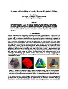
Figure 1 Left-hand side: the pentagrid. Right-hand side: the heptagrid. tessellation starting from a regular polygon. This means that, starting from the polygon, we recursively copy it by reflections in its sides and of the images in their sides. This family of tilings is defined by two parameters: p, the number of sides of the polygon and q, the number of polygons which can be put around a vertex without overlapping and covering any small enough neighbourhood of the vertex. In order to represent the tilings which we shall consider and the regions whose contour word will be under study, we shall make use of the Poincar´e’s disc model. Our illustrations will take place in the pentagrid and the heptagrid, i.e. the tilings {5, 4} and {7, 3} respectively of the hyperbolic plane. Figures 1 and 2 illustrate these tilings.
Hyperbolic tilings and formal language theory
130
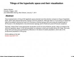
Figure 2 Left-hand side: the pentagrid. Right-hand side: the heptagrid. Note that in both cases, the sectors are spanned by the same tree. 1
1 2
3
1 0 0
1 0 5
6
1 0 0 0
1 0 0 0 0 0
1 0 0 0 0 1
1 0 0 0 1 0
7
1 0 0 1
13 14 15 16
1 0 0 1 0 0
8
1 0 1 0
1 0 1 0 0 0
1 0 1 0 0 1
1 0 1 9
1 0 0 0 0
17 18 19 20
1 0 0 1 0 1
4
10
1 0 0 0 1
21 22 23 24 25
1 0 1 0 1 0
1 0 0 0 0 0 0
1 0 0 0 0 0 1
1 0 0 0 0 1 0
11
1 0 0 1 0
1 0 0 0 1 0 0
12
1 0 1 0 0
1 0 1 0 1
26 27 28 29
1 0 0 0 1 0 1
1 0 0 1 0 0 0
1 0 0 1 0 0 1
1 0 0 1 0 1 0
30 31 32 33
1 0 1 0 0 0 0
1 0 1 0 0 0 1
1 0 1 0 0 1 0
1 0 1 0 1 0 0
1 0 1 0 1 0 1
Figure 3 The standard Fibonacci tree. The nodes are numbered from the root, from left to right on each level and level after level. For each node, the figure displays the representation of the number of the node with respect to the Fibonacci sequence, the representation avoiding consecutive 1’s.
From Figure 1,the pentagrid and the heptagrid seem rather different. However, there is a tight connection between these tilings which can be seen from Figure 2. In both pictures of the latter figure, we represent the tiling by selecting a central tile and then, by displaying as many sectors as the number of sides of the central tile. In each case, these sectors do not overlap and their union together with the central cell gives the tiling of the whole hyperbolic plane. Now, there is a deeper common point: in both cases, each sector is spanned by a tree which we call a Fibonacci tree for a reason which will soon be explained. As proved in [6, 9], the corresponding tree can be defined as follows. We distinguish two kinds of nodes, say black nodes, labelled by B, and white nodes, labelled by W . Now, we get the sons of a node by the following rules: B → BW and W → BWW , the root of the tree being a white node, see Figure 3. It is not difficult to see that if the root is on level 0 of the tree, the number of nodes on the level k of the tree is f2k+1 , where { fk }k∈IN is the Fibonacci sequence with f0 = f1 = 1. The Fibonacci tree has a lot of nice properties which we cannot discuss here. In particular, there is a way to locate the tiles of the pentagrid or the heptagrid very easily thanks to coordinates devised from the properties of the Fibonacci tree, see [6, 9, 10].
M. Margenstern, K.G. Subramanian
4
131
Grammars
As mentioned in the introduction, the tilings considered in Section 3 can be generated by a grammar. Consider the case of the pentagrid. Then its spanning tree can be generated by the following grammar: symbols: X , Y , Z, C, W , B, with C, W and B being terminals; initial symbol: Z; (G0 ) rules: Z ⇒ CYYYYY Y ⇒ W XYY X ⇒ BXY Indeed, in the above rules, the symbol ⇒ is interpreted as follows: the tile which is on the left-hand side of the ⇒ is replaced by the set of tiles which is indicated in the right-hand side of the ⇒. In all cases, this right-hand side set of tiles is a finite tree which consists of a root with its sons. The root is the leftmost letter and the sons are the following letters given in the order in the tree from left to right. Note that this grammar is deterministic. Also note that the generation process may vary: the replacement of the variables can be performed uniformly level by level, it can be also performed following other rules. Also note that this grammar allows us to reproduce the tree structure of the tessellation. If we wish to cover the plane only, we can simplify the grammar to: symbols: X , Y , Z, T , with T being terminal; initial symbol: Z; (G1 ) rules: Z ⇒ TYYYYY Y ⇒ T XYY X ⇒ T XY In [6], we considered other substitutions as, for instance, this one: symbols: X , Y , Z, C, W , B, with C, W and B being terminals; initial symbol: Z; (G2 ) rules: Z ⇒ CYYYYY Y ⇒ WY XY X ⇒ BXY keeping the indication of the tree structure. Here, we obtain a different tree than the one attached to the previous grammar. However, it spans the same tessellation if we erase the difference between C, W and B. Now, in [6], we proved that in fact, we have six possible set of rules, considering that for X we have two possible rules: X ⇒ BXY and X ⇒ BY X and that for Y , we have three of them: Y ⇒ BXYY , Y ⇒ BY XY and X ⇒ BYY X We also proved that while replacing the variable by a symbol by the application of a rule, we could switch from one set of rules to another at random: we obtain an uncountable set of trees spanning the
132
Hyperbolic tilings and formal language theory
tessellation but we still obtain the same tessellation, once the colours of the tiles are forgotten. This process can be described by a single grammar: symbols: X , Y , Z, T , with C, W and B being terminals; initial symbol: Z; rules: (G3 ) Z ⇒ CYYYYY Y ⇒ W XYY | WY XY | WYY X X ⇒ BXY | BY X This time, the grammar is non-deterministic and this relaxation of determinism allows us to handle in a more synthetic expression a process which would require more elaboration using the single notion of substitution. Last remark on the generation of the tessellation: using substitution or grammars, the tessellation itself is obtained after using infinitely many applications of the rules. Finitely many applications always lead to a finite figure whose size increases with the number of applications. Also note that if we apply only rules with Y , we get binary trees. If we apply only rules with X , we get six lines of X with, for each X -line, a kind of shadow consisting of Y ’s. The grammars (G1 ) up to (G3 ) can be generalized to the tilings studied in [2] and [8], the tessellations {5, 3, 4} and {5, 3, 3, 4}. This can also be generalized more easily with the tilings {p, 4} and {p+2, 3} when p ≥ 5. For the same value of p, the tessellations {p, 4} and {p+2, 3} are generated by the same tree which generalizes the Fibonacci tree. The generalizations of (G1 ) are of the form: symbols: X , Y , Z, C, W , B, with C, W and B being terminals; initial symbol: Z; (G p ) rules: Z ⇒ CY p Y ⇒ W XY p−3 X ⇒ BXY p−4 Again, we can define p−3 rules for Y and p−4 rules for X and, as above, a non-deterministic grammar which can generate uncountably many trees, each one generating the considered tessellation.
5
Contour words and words along a level
In [11], the first author considered the possibility to define words by looking at a specific object: the set of tiles which lie at a given distance from another tile, fixed in advance and once for all. Fix a tile C which will later be called the central one. A path from a tile T to C is a finite sequence Ti , 0 ≤ i ≤ n of tiles such that T0 = C, Tn = T and for all i in [0..n−1], Ti ∩ Ti+1 consists of one edge exactly. Then we say that n is the length of the path. The distance from T to C is the shortest length for a path joining T to C. Clearly, the distance is always defined. Now, a ball B around C of radius ρ is the set of tiles T whose distance to C is at most ρ . The border of B, centered at C and denoted by ∂ B is the set of tiles whose distance to C is the radius of B. Consider Γ a grammar defined in Section 4. Then, we call Γ-contour word the set of words obtained by taking the restriction of a tiling generated by Γ with Z at the central tile C on the border of a ball of radius n around C. As proved in [11], the set of these words is generated by a 2-iterated pushdown automaton. We reproduce the algorithm which proves this property in Automaton 2. It was also mentioned
M. Margenstern, K.G. Subramanian
133
in [11] that a simple application of Ogden’s pumping lemma shows that the set of these words cannot be generated by a pushdown automaton.
Figure 4 Levels in the heptagrid. Automaton 2 The 2-pushdown automaton recognizing the contour word of a ball in the pentagrid or in the heptagrid.
two states: q0 and q1 ; input word in {b, w}∗ ; Γ = {Z, B,W, F }; initial state: q0 ; initial stack: Z[ε ]; transition function δ :
δ (q0 , ε , Z) = {(q0 , push2 (F)), (q0 , push1 (W α ))} δ (q0 , ε , ZF) = {(q0 , push2 (FF)), (q0 , push1 (W α ))} δ (q0 , ε ,W F) = (q1 , pop2 ) δ (q0 , ε , BF) = (q1 , pop2 ) δ (q0 , b, B) = (q0 , pop1 ) δ (q0 , w,W ) = (q0 , pop1 ) δ (q1 , ε ,W F) = (q0 , push1 (BWW )) δ (q1 , ε , BF) = (q0 , push1 (BW )) δ (q1 , ε ,W ) = (q0 , push1 (BWW )) δ (q1 , ε , B) = (q0 , push1 (BW )) Now, it was proved in [9] that the set of tiles which are on the same level in a Fibonacci tree belong to a part of the border of a ball around the root of the Fibonacci tree. Consider again a fixed ball around C and fix one of the finite Fibonacci trees generated around C, say F . We can imagine C as the central tile in Figure 5. Let B the ball around C which contains F and whose border contains the leaves of F . It is not difficult to find a tile C1 which is a neighbour of C and such that C1 is the root of a Fibonacci tree F1 in the ball B1 around C1 containing F . We can assume that, in the same way, the border of B1 contains the leaves of F1 . In Figure 5, left-hand side picture, we have a line δ1 which passes through the mid-points of consecutive edges of heptagons. We define C1 as the yellow neighbour of C which is cut by δ1 and which is above C. We can remark that C is the image of C1 by a shift along the line δ1 . Now, it is not difficult to see that the restriction of the tiling to F1 contains the restriction of the tiling to F . We can also see
Hyperbolic tilings and formal language theory
134
that the leaves of F are contained in those of F1 . In the left-and side picture of Figure 5, the sector generated by a black tile is delimited by the ray a and the line δ1 . The two sectors generated by a white tile are delimited by the line δ1 and the ray b and then by the ray b and the ray e. A similar convention is followed for the tree rooted at C1 : the rays a1 , b1 and e1 play the same role for C1 as the rays a, b and e for C. From the figure, it is not difficult to see that, by induction, we construct a sequence of tiles Cn with C0 a tile crossed by δ1 and which is fixed once and for all, Cn+1 , n ≥ 0, is the neighbour of Cn which is crossed by δ1 and which is defined by the fact that its distance from C0 is n+1 and by the fact that Cn is in between Cn+1 and C0 . We define Bn as the ball around Cn whose border contains C0 and Fn is the Fibonacci tree rooted at Cn whose leaves are on Bn . This allows us to define a sequence of words wn which is the trace of the leaves of Fn : wn is in {B,W }⋆ and the jth letter of wn is B, W , depending on whether the jth leave of Fn is black, white respectively. The construction shows us that wn is a factor of wn+1 and we may assume that there are nonempty words un and vn such that wn+1 = un wn vn . A closer look at the construction indicated in Section 4 shows that vn = wn and that un+1 = un wn . Indeed, the separation between un and wn vn = wn wn is materialized by δ1 . Note that the separation between the two occurrences of wn is not fixed: it moves and tends to infinity as the length of wn itself tends to infinity. And so, wn is defined at the same time as un by the two equations: wn+1 = un wn wn un+1 = un wn with initial conditions u0 = B and w0 = W . As the lengths of un and wn tend to infinity, and as δ1 is fixed, we can see from the left-hand side picture of Figure 5 that the sequence of words wn tend to a bi-infinite word, i.e. a word whose both ends tend to infinity.
e1
e e1
b1 C1
C1 a1
b
C
C δ2
δ1 a1
e
a b
a
Figure 5 Heptagrid: construction of bi-infinite words. Left-hand side: the bi-infinite word associated with the grammar (G1 ). Right-hand side: the bi-infinite word associated with the grammar (G2 )
In the right-hand side picture of Figure 5, we have a similar construction with the grammar (G2 ). Presently, define xn and yn as the words defined by the trace of the leaves of the tree constructed according to the rules of (G2 ) with x0 = B and y0 = W . Then, the equations satisfied by xn and yn are: yn+1 = yn xn yn xn+1 = xn yn
M. Margenstern, K.G. Subramanian
135
Note that these words are very different from the wn ’s and the un ’s. We can see that, this time, the sectors are delimited in a different way: the rays a and b are not on the same side with respect to δ1 . On the figure, we can see that the sectors are delimited as follows: a and δ2 delimit a white sector, then δ2 and the ray b delimit the black sector and, again, we have a white sector delimited by b and e. These rays are used for the tree rooted at C. Similar rays, a1 , b1 and e1 are used for the tree rooted at C1 : as can be seen on the figure, the tree contains the one defined from C. Note that b1 is the continuation of e. As in the case with the left-hand side picture, this picture also defines a bi-infinite word as the limit of wn . Note that, in both case, un tends to a limit which is infinite on one side only: this can be seen by the fact that the black sector is always delimited by δ1 or δ2 and these lines are fixed. The infinite limit is finite to the left in the case of (G1 ), it is finite to the right in the case of (G2 ).
e1 C1
δ1
e1
b1
b1 C1
e δ2
C
e
C
b
b
a a
Figure 6 Heptagrid: construction of one-sided infinite words. Left-hand side: an infinite word associated with the grammar (G1 ), Right-hand side: an infinite word associated with the grammar (G2 )
In both cases, say that δ1 and δ2 are separators: δ1 separates un from wn wn for each n; δ2 separates yn from xn yn . Figure 6 illustrates a similar construction leading to an infinite limit for wn which is infinite on one side only. The rays a, b and e play similar roles with the lines δ1 or δ2 as in the Figure 5. Note that in the left-hand side picture, a1 is not mentioned as it contains the ray b. In the right-hand side picture, the ray a1 coincide with the ray e. From the picture, it is clear that this time the limit of wn and that of yn are both infinite to the right. In the case of (G1 ), the limit of un is also infinite to the right only. In the right-hand side picture, we can see that the different terms xn are disjoint. However, each one is the same asi un with the same index in the left-hand side picture: accordingly, the limit is the same. Other constructions of the same type, with again a fixed separator between both occurrences of wn in the case of G1 and in between un and wn in the second case lead to different pictures and to other infinite words. We leave them as an exercise to the reader.
Acknowledgment The second author acknowledges support by the project Universit´e de la Grande R´egion UniGR that enabled his visit during February 2013, in particular at LORIA, Universit´e de Lorraine, France.
136
Hyperbolic tilings and formal language theory
References [1] S. Fratani G. S´enizergues (2006): Iterated pushdown automata and sequences of rational numbers. Annals of pure and applied logic 141, pp. 363–411, doi:10.1016/j.apal.2005.12.004. [2] M. Margenstern G. Skordev (2003): Tools for devising cellular automata in the hyperbolic 3D space. Fundamenta Informaticae 58(2), pp. 369–398. [3] C. Goodman-Strauss (2009): Regular production systems and triangle tilings. Theoretical Computer Science 410, pp. 1534–1549, doi:10.1016/j.tcs.2008.12.012. [4] S. Greibach (1970): Full AFL’s and nested iterated substitution. Information and Control 16(1), pp. 7–35, doi:10.1016/s0019-9958(70)80039-0. [5] A.V. Kelarev (2003): Graph Algebras and Automata. Marcel Dekker, New York. [6] M. Margenstern (2000): New Tools for Cellular Automata of the Hyperbolic Plane. Journal of Universal Computer Science 6(12), pp. 1226–1252, doi:10.3217/jucs-006-12-1226. [7] M. Margenstern (2002): Tiling the hyperbolic plane with a single pentagonal tile. Journal of Universal Computer Science 8(2), pp. 297–316, doi:10.3217/jucs-008-02-0297. [8] M. Margenstern (2004): The tiling of the hyperbolic 4D space by the 120-cell is combinatoric. Journal of Universal Computer Science 10(9), pp. 1212–1238, doi:10.3217/jucs-010-09-1212. [9] M. Margenstern (2007): Cellular Automata in Hyperbolic Spaces, volume I : Theory, first edition. Advances in Unconventional Computing and Cellular Automata, Editor: Andrew Adamatzky 1, Old City Publishing´ Edition des archives contemporaines, Philadelphia, PA, USA - Paris, France. [10] M. Margenstern (2008): Cellular Automata in Hyperbolic Spaces, volume II : Implementation and Computations, first edition. Advances in Unconventional Computing and Cellular Automata, Editor: Andrew ´ des archives contemporaines, Philadelphia, PA, USA - Paris, Adamatzky 2, Old City Publishing-Edition France. [11] M. Margenstern (2012): An Application of Iterative Pushdown Automata to Contour Words of Balls and Truncated Balls in Hyperbolic Tessellations. ISRN Algebra 2012, p. 14p, doi:10.5402/2012/742310. [12] A.N. Maslov (1974): The hierarchy of indexed languages. Soviet Mathematics, Doklady 15, pp. 1170–1174.