An algorithmic approach to tilings of hyperbolic spaces: 10 ... - CMC11

An algorithmic approach to tilings of hyperbolic spaces: 10 years later Maurice Margenstern Universit´ e de Metz, LITA, EA 3097

CMC’11 August, 24-27, 2010 JENA, GERMANY

in this talk: 1. hyperbolic geometry: what to know 2. navigation in hyperbolic spaces 3. application to hyperbolic tilings 4. application to hyperbolic CA’s 5. present applications and future ones

1. hyperbolic geometry: what to know

hyperbolic geometry = absolute geometry + new axiom (Lobachevsky-Bolyai): from a point A out of a line L, at least two parallels to L extension to any dimension many models: Beltrami, Klein, Poincar´ e,...

Poincar´ e’s disc model

the disc


a point A A


a point A a line ℓ

A

l


a secant through A which cuts ℓ

A

s l


a parallel p to ℓ through A

A

p

s l

P


another parallel q to ℓ through A

A q p

s l Q

P


a non secant line m to ℓ through A

m A q p

s l Q

P


h

the common perpendicular to ℓ and to m

m A q p

s l Q

P

a few useful properties the sum of angles in a triangle: always less than π non-secant lines : always a unique common perpendicular no similarity in the Euclidean meaning

2. navigation in hyperbolic spaces

2.1 tessellations in hyperbolic spaces 2.2 a GP S for the hyperbolic plane 2.3 generalization to many hyperbolic grids 2.4 generalization to the third and the fourth dimensions

2.1 tessellations in hyperbolic spaces tessellations in the plane: let P be a regular polygon reflect P in its sides and recursively, the images in their sides, say copies of P we get a tessellation if and only if the copies do not overlap and their union is the plane

in the Euclidean plane, there are 3 tessellations, up to similarity: the square, the hexagonal and the triangular grids

in the hyperbolic plane, there is an important result: theorem (Poincar´ e, 1882) any trian2π 2π 2π , and , with gle with angles p q r p, q and r positive integers such that 1 1 1 1 + + < p q r 2 defines a tessellation of the hyperbolic plane

accordingly, infinitely many tessellations in particular, based on the rectangle

π π and : triangle with acute angles p q

= tessellation on the regular polygon with p sides and q polygons around a vertex notation: {p, q}

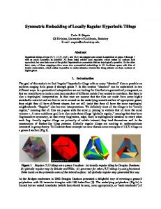
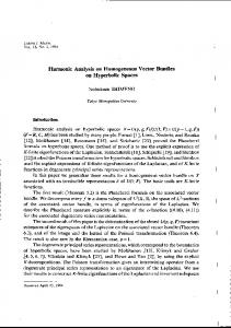
illustration of two grids of the hyperbolic plane

the pentagrid and the heptagrid

{5, 4}

{7, 3}

2.2 a GP S for the hyperbolic plane first, in the pentagrid, tessellation of the regular rectangular pentagon look at a quarter of the plane:

2.2 a GP S for the hyperbolic plane first, in the pentagrid, tessellation of the regular rectangular pentagon now with the generating tree:

second, same property in the heptagrid, tessellation of the regular hep2π tagon with angle : 3 the same generating tree:

the splitting process for the pentagrid:

the leading pentagon P of a quarter


in the complement of P a quarter


another one


and the remaing part: a strip


in a strip: the leading pentagon and a quarter


the remaing part: a strip again


the recursive splitting: first step


the recursive splitting: second step


the recursive splitting: third step


and so we get the announced bijection of the tiling on the quarter with a tree

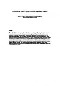
the Fibonacci technology the Fibonacci tree: 1

1 2

3

4

1 0 5

6

14 15

1 0 0 0 0 0

1 0 0 0 0 1

1 0 0 0 1 0

7

1 0 0 1

1 0 0 0 13

1 0 0

16

1 0 0 1 0 0

17

1 0 0 1 0 1

18

1 0 1 0 0 0

19

1 0 1 0 0 1

8

9

1 0 0 0 0

20 21

22

1 0 0 0 0 0 0

10

1 0 0 0 0 0 1

23

1 0 0 0 0 1 0

11

24

1 0 0 0 1 0 0

25

1 0 0 0 1 0 1

12

1 0 1 0 1

1 0 1 0 0

1 0 0 1 0

1 0 0 0 1

1 0 1 0

1 0 1 0 1 0

1 0 1

26

1 0 0 1 0 0 0

27 28

1 0 0 1 0 0 1

1 0 0 1 0 1 0

29

1 0 1 0 0 0 0

30

1 0 1 0 0 0 1

31

1 0 1 0 0 1 0

32

1 0 1 0 1 0 0

33

1 0 1 0 1 0 1

the key property let αk . . . α0 be the coordinate of ν and let βh . . . β0 represent ν−1 coordinates of the sons of ν: if ν 2-node: αk . . . α000 ,

αk . . . α001

if ν 3-node: βh . . . β010 ,

αk . . . α000 ,

αk . . . α001

call the node with coordinate the preferred son of ν

αk . . . α000

every node has precisely one preferred node: in 2-nodes, the leftmost son in 3-nodes, the middle one

an important property: the language of the coordinates is regular this explains the following result: theorem (MM, 2003) − in the Fibonacci tree, there is an algorithm to compute the path from a node ν to the root, linear in the coordinate of ν

3. application to hyperbolic tilings

3.1 the splitting method 3.2 paying a visit to the hyperbolic 3D 3.3 the hyperbolic 4D 3.4 undecidability of the tiling problem 3.5 related tiling problems

3.1 the splitting method

the method generalizes the slpitting of the pentagrid or of the heptagrid the Fibonacci technology also generalizes to a wider context

basis of splitting assumed: k unbounded simply connected parts of IH n: S0, . . ., Sk , and h bounded simply connected parts of IH n, P0, . . ., Ph, h ≤ k, with:

(i) IH n split into finitely many copies of S0 (copy = isometric image)

(ii) each Si split into one copy of some Pℓ and finitely many copies of Sj distinguished Pℓ: leading tile of Si

the spanning tree of the tiling root : the leading tile of S0 let level n defined and each node associated to the leading tile of a copy Cj of some Sj then, sons of leading tile of Cj : leading tiles of copies of those Sk ’s occurring in the splitting of Cj by induction: infinite tree

combinatoric tilings the tiling T is combinatoric if there is a basis of splitting such that: the spanning tree is in bijection with the restriction of T to S0, all tiles of T being copies of Pℓ’s later, in most cases, a single generating tile P = P0

matrix and polynomial of the splitting when combinatoric tiling, the spanning tree has k+1 types of nodes: type i means Si moreover: let Mi,j = {#Sj in splitting Si}; ⇒ the number of nodes of level n for a root of type i = sum of row i+1 of M n

M : matrix of the splitting; its characteristic polynomial: polynomial of the splitting

language of the splitting let un = #{ nodes at level n of A} with A spanning tree

{u}n satisfies the induction equation defined by the polynomial of the splitting number the nodes of A starting from 1, from the root and level by level: coordinate of node ν = maximal greedy representation of ν language of the splitting = language of the coordinates

greedy representation in a basis let {un}n∈IN be positive numbers with

un

u0 = 1, un < un+1 and limsup 0, the radius here, k = 1, also most studied case so, around c : c−1, c, c+1

format of the rules: the rules are written: η−1η00η1 → η01 with η−1, state of cell c−1, η00, current state of cell c η1, state of cell c+1, η01, new state of cell c also written as: η−1 η00 η01

η1

universality on 1D CA’s it is easy to prove that among 1D CA’s, there are universal ones the idea: simulate any Turing machine the key point: the Turing tape is the CA

implementation of the idea: for each cell of the CA: state: the content of the square of the Turing tape automaton: the program of the Turing machine

a precise elementary result for universality: theorem let M be a Turing machine with m letters and n states; then M can be simulated by a 1D CA which has m+2n states using the smallest known Turing machines, this gives us 15 states

easy proof simulating an instruction with a move to right: before: u α p β γ v after:

u α δ q γ v

whence the rules: α p α α

p β β β

β γ γ p

→ → → →

δ q β β

simulating an instruction with a move to left: before: u α p β γ v after:

u α q’ δ γ v u q α δ γ v

whence the rules: α p β → q’ p β γ → δ α β γ → β

α β q’ → q’ α q’ δ → α α β p → β

up to now, classical setting of the initial configuration: there is a quiescent state q, called blank with the rule: q q q → q and, all cells except finitely many of them are initially blank

weak universality on 1D CA’s the initial configuration may have infinitely many blank cells, but it may not be arbitrary: the initial configuration must be a regular language

elementary CA’s there are 1D CA’s with 2 states, 0 and 1, or and read the neighbourhood as the binary representation of a number in {0..7} each rule associates 0 or 1 to a number in {0..7}

hence, the set of rules can be represented by a mapping f from {0..7} into

{0, 1} order the neighbours n0, ..., n7 by the natural order on their numbers then, f (n0), ..., f (n7) can be read as the binary representation of a number in {0..255} which is the number of the set of rules, in short, number of the rule

rule 110

rule 110 gives rise to very complexed patterns

already starting from a single cell in :

space-time diagram of rule 110 starting from a configuration with a single cell in 1

same starting point after 150 iterations:

one of the key patterns of rule 110:

theorem (Matthiew Cook, 2004) − rule 110 is weakly universal weak universality of rule 110: conjectured by Stephen Wolfram in 1985

Euclidean 2D CA’s

we consider the square grid which is identified with Z Z 2, the most studied grid now, traditionally, there are two kinds of neighbourhoods: von Neumann neighbourhood Moore neighbourhood

von Neumann neighbourhood

assume the central cell to be (0,0) the neighbours are: N, W, S, E (0,1), (−1,0) (0,−1), (0,1)

representation of the von Neumann neighbourhood of a cell

Moore neighbourhood

assume the central cell to be (0,0) the neighbours are N, W, S, E and: NW, SW, SE, NE (−1,1), (−1,−1) (−1,1), (1,1)

representation of the Moore neighbourhood of a cell

universality on 2D CA’s an important result is given by the following statement: theorem (E.F. Codd, 1968) − for a CA on the square grid with 2 states and starting from a finite configuration, the halting problem is decidable if the cells have at most five neighbours

as a consequence, there are no universal CA on the plane with 2 states and with von Neumann neighbourhood another consequence: rule 110 is weakly universal but it is not strongly universal

weak universality on 2D CA’s there is a well known result: theorem (Berlekamp, Conway, Guy, 1982) Conway’s game of life is weakly universal the game of life is a CA on the square grid with 2 states and Moore neighbourhood, Conway, 1972

4.2. implementing CA’s in hyperbolic spaces

format of rules for hyperbolic CA’s fix a central cell and dispatch α sectors around it, α ∈ {5, 7}:

1

1

5

7

2

2

4 3

6 3

5 4

number the sectors from 1 to α, counterclockwise then, coordinate of a cell:

(ν, σ) with ν , coordinate in the tree and σ , number of the tree

the local numbering number the sides of a tile from 1 to α while clockwise turning around the tile number 1: if central cell: side to a fixed in advance neighbour if not central cell: side to the father

η0: current state of the cell ηi: state of the neighbour i, seen from the side i, ∈ {1..α} η01: new state of the cell format of a rule: η0η1...ηα → η01 1a for short η0η1...ηαη0

η0η1...ηα: context of the rule

4.2 general results

the global function of a CA Euclidean case: consider a CA A on Z Z d , d ≥ 1, define:

Q, the states, N the neighbourhood,

fA, the transition function

d Z Z the set of configurations of A is Q d Z Z by: fA defines GA on Q

∀x GA(c)(x) = fA(c(x+N )) GA is the global function of fA

theorem (Curtis, Hedlund, Lyndon − 1969) d Z Z a function F from Q into itself is the global function of a cellular automaton A with a ball as the neighbourhood if and only if: d Z Z • F is continuous when Q is endowed with the product topology • F commutes with the shifts

in the hyperbolic plane: theorem (MM, 2008) a function F from Q1+αF into itself is the global function of a rotation invariant cellular automaton A with a ball as the neighbourhood if and only if: • F is continuous when Q1+αF is endowed with the product topology • F commutes with the shifts where F is the Fibonacci tree

theorem (Moore, 1962, Myhill, 1963) let A be a cellular automaton on the Euclidean plane; then GA is surjective if and only if it is injective on finite configurations theorem (Kari, 1994) it is undecidable to know whether the global function of a CA on the Euclidean plane is injective

in the hyperbolic plane theorem (Kari, MM, 2009) there are CA’s on the pentagrid or on the heptagrid whose global function is injective on finite configurations but not surjective and there are also CA’s on the pentagrid and on the heptagrid whose global function is surjective but not injective on finite configurations

we also have: theorem (MM, 2008) it is undecidable to know whether the global function of a CA on the pentagrid or the heptagrid is injective

4.3 complexity results for hyperbolic CA’s

a precursor result

theorem Morgenstein-Kreinovich, 1995 NP-hard problems can be solved in polynomial time in a hyperbolic space note that in this paper there is no explicit construction

the pioneer result theorem MM-Morita, 1999 there is a CA on the pentagrid which can solve SAT in quadratic time remarks: the Fibonacci technology did not yet exist in fact, the estimate is very rough: the considered CA works in linear time

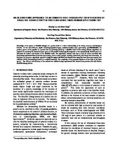
the key idea: 11 00 00 11

11 00 00 11

000 111 000 111 000 111 000 111 000 111 1111111111111111 00 11 0000000000000000 000 111 000 111 000 111 000 111 000 111 00 11 0000000000000000 1111111111111111 00 11 0000000000000000 1111111111111111 00 11 0000000000000000 1111111111111111 00 11 0000000000000000 1111111111111111 000 111 00000000 11111111 000000000 111111111 00000000000000 11111111111111 000 111 00000000 11111111 000000000 111111111 00000000000000 11111111111111 000 111 00000000 11111111 000000000 111111111 00000000000000 11111111111111 000 111 00000000 11111111 000000000 111111111 00000000000000 11111111111111 000 111 00000000 11111111 000000000 111111111 00000000000000 11111111111111 00000 11111 000 111 00000000 11111111 00000 11111 00000 11111 000 111 00000000 11111111 00000 11111 00000 11111 000 111 00000000 11111111 00000 11111 00000 11111 000 111 00000000 11111111 00000 11111 00000 11111 000 111 00000000 11111111 00000 11111 00000 11111 000 111 00000000 11111111 00000 11111 00000 11111 000 111 00000000 11111111 00000 11111 00000 11111 000 111 00000000 11111111 00000 0000011111 11111 000 111 00000000 11111111 00000 0000011111 11111 000 111 00000000 11111111 00000 11111

00 11 00 11 00 11 00 11 11 00 000 00000 11111 000000 111111 111111 000000 1111111111111111 0000000000000000 00111 11 00 11 00 11 000 111 00000 11111 000000 111111 111111 000000 1111111111111111 0000000000000000 00 11 000 111 00000 11111 000000 111111 111111 000000 1111111111111111 0000000000000000 00 11 000 111 00000 11111 000000 111111 111111 000000 1111111111111111 0000000000000000 00 11 000 111 00000 11111 000000 111111 111111 000000 1111111111111111 0000000000000000 00 11 000 111 00000 11111 000000 111111 111111 000000 1111111111111111 0000000000000000 00 11 000 111 00000 11111 000000 111111 111111 000000 1111111111111111 0000000000000000 00 11 000 111 00000 11111 000000 111111 111111 000000 1111111111111111 0000000000000000 00 111 11 000 00000 11111 000000 111111 111111 000000 1111111111111111 0000000000000000 00 11 00 11 00 11 00 11 00 11 00 11 00 11 00 11 0000000 1111111 0000000 1111111 0000000 1111111 0000000 1111111 111111 000000 1111 0000 1111 0000 111111111 11111111111111 1111 000000000 00000000000000 0000 00 11 00 11 00 11 00 11 0000000 1111111 0000000 1111111 0000000 1111111 0000000 1111111 111111 000000 1111 0000 1111 0000 111111111 11111111111111 1111 000000000 00000000000000 0000 0000000 1111111 0000000 1111111 0000000 1111111 0000000 1111111 111111 000000 1111 0000 1111 0000 111111111 11111111111111 1111 000000000 00000000000000 0000 0000000 1111111 0000000 1111111 0000000 1111111 0000000 1111111 111111 000000 1111 0000 1111 0000 111111111 11111111111111 1111 000000000 00000000000000 0000 0000000 1111111 0000000 1111111 0000000 1111111 0000000 1111111 111111 000000 1111 0000 1111 0000 111111111 11111111111111 1111 000000000 00000000000000 0000 0000000 1111111 0000000 1111111 0000000 1111111 0000000 1111111 111111 000000 1111 0000 1111 0000 111111111 11111111111111 1111 000000000 00000000000000 0000 0000000 1111111 0000000 1111111 0000000 1111111 0000000 1111111 111111 000000 1111 0000 1111 0000 111111111 11111111111111 1111 000000000 00000000000000 0000 0000000 1111111 0000000 1111111 0000000 1111111 0000000 1111111 111111 000000 1111 0000 1111 0000 111111111 11111111111111 1111 000000000 00000000000000 0000 0000000 1111111 0000000 1111111 0000000 1111111 0000000 1111111 111111 000000 1111 0000 1111 0000 111111111 11111111111111 1111 000000000 00000000000000 0000 00 11 00 11 00 11 00 11 00 11 00 11 00 11 00 11 00 11 00 11 00 11 00 11 00 11 00 11 00 11 00 11 00 11 00 11 0000 1111 00000 11111 000000 111111 111111111 000000000 0000000 111111 000000 1111 0000 0 1111 0000 1 0 000 111 000 111 000 111 000 000 11111 111 00000 000 111 11111 11111111 000 00000 00000000 00 11 00 1111111 11 00 1 11 00 111 11 00 11 00 11 00 111 11 00 11 00 11 0000 1111 00000 11111 000000 111111 111111111 000000000 1111111 0000000 111111 000000 1111 0000 1 0 1111 0000 1 0 111 000 111 000 111 000 111 000 111 000 11111 111 00000 000 111 11111 11111111 000 00000 00000000 0000 1111 00000 11111 000000 111111 111111111 000000000 1111111 0000000 111111 000000 1111 0000 1 0 1111 0000 1 0 111 000 111 000 111 000 111 000 111 000 11111 111 00000 000 111 11111 11111111 000 00000 00000000 0000 1111 00000 11111 000000 111111 111111111 000000000 1111111 0000000 111111 000000 1111 0000 1 0 1111 0000 1 0 111 000 111 000 111 000 111 000 111 000 11111 111 00000 000 111 11111 11111111 000 00000 00000000 0000 1111 00000 11111 000000 111111 111111111 000000000 1111111 0000000 111111 000000 1111 0000 1 0 1111 0000 1 0 111 000 111 000 111 000 111 000 111 000 11111 111 00000 000 111 11111 11111111 000 00000 00000000 0000 1111 00000 11111 000000 111111 111111111 000000000 1111111 0000000 111111 000000 1111 0000 1 0 1111 0000 1 0 111 000 111 000 111 000 111 000 111 000 11111 111 00000 000 111 11111 11111111 000 00000 00000000 0000 1111 00000 11111 000000 111111 111111111 000000000 1111111 0000000 111111 000000 1111 0000 1 0 1111 0000 1 0 111 000 111 000 111 000 111 000 111 000 11111 111 00000 000 111 11111 11111111 000 00000 00000000 0000 1111 00000 11111 000000 111111 111111111 000000000 1111111 0000000 111111 000000 1111 0000 1 0 1111 0000 1 0 111 000 111 000 111 000 111 000 111 000 11111 111 00000 000 111 11111 11111111 000 00000 00000000 0000 1111 00000 11111 000000 111111 111111111 000000000 1111111 0000000 111111 000000 1111 0000 1 0 1111 0000 1 0 111 000 111 000 111 000 111 000 111 000 11111 111 00000 000 111 11111 11111111 000 00000 00000000 00 11 00 11 00 11 00 11 00 11 00 11 00 11 00 11 00 11 00 11 00 11 00 11 00 11 00 11 00 11 00 11 00 11 00 11 00 11 00 11 00 11 00 11 00 11 00 11 00 11 00 11 00 11 00 11 00 11 00 11 00 11 00 00 00 00 11 00 11 00 11 00 11 00 11 11 00 11 00 11 00 11 00 11 00 11 00 00 11 11 00 11 00 11 00 11 11 00 11 11 00 11

11 00 00 11

11 00 00 11

11 00 00 0011 11 00 11

11 00 00 00 11 11 00 11

11 00 00 11

binary representation of the data

the key idea: 11 00 00 11 00 11

11 00 00 11 00 11

unary representation of the data

11 00 00 11 00 11

00 11 11 00 00 11

11 00 00 11 00 11

11 00 00 11 00 11

11 00 00 11 00 11

11 00 00 11 00 11 11 00 00 11 00 11

111110000 00000 11110000 11110000 11110000 111100000 11111 000 111 000 000 000 000 1111111111111111 00 11 0000000000000000 000 111 111 000 111 111 000 111 111 000 111 111 000 111 00 11 0000000000000000 1111111111111111 00 11 0000000000000000 1111111111111111 00 11 0000000000000000 1111111111111111 00 11 0000000000000000 1111111111111111 000 111 00000000 11111111 000000000 111111111 00000000000000 11111111111111 000 111 00000000 11111111 000000000 111111111 00000000000000 11111111111111 000 111 00000000 11111111 000000000 111111111 00000000000000 11111111111111 000 111 00000000 11111111 000000000 111111111 00000000000000 11111111111111 000 111 00000000 11111111 000000000 111111111 00000000000000 11111111111111 00000 11111 000 111 00000000 11111111 00000 11111 00000 11111 000 111 00000000 11111111 00000 11111 00000 11111 000 111 00000000 11111111 00000 11111 00000 11111 000 111 00000000 11111111 00000 11111 00000 11111 000 111 00000000 11111111 00000 11111 00000 11111 000 111 00000000 11111111 00000 11111 00000 11111 000 111 00000000 11111111 00000 00000 11111 000 111 00000000 11111111 00000 0000011111 11111 000 111 00000000 11111111 00000 11111 0000011111 11111 000 111 00000000 11111111 00000 11111

111111 000000 1111111111111111 0000000000000000 111111 000000 1111111111111111 0000000000000000 111111 000000 1111111111111111 0000000000000000 111111 000000 1111111111111111 0000000000000000 111111 000000 1111111111111111 0000000000000000 111111 000000 1111111111111111 0000000000000000 111111 1111111111111111 000000 0000000000000000 111111 000000 1111111111111111 0000000000000000 111111 000000 1111111111111111 0000000000000000 00 11 00 11 00 11 00 11 00 11 00 11 000000 111111 000000 111111 000000 111111 000000 111111 111111 000000 1111 0000 1111 0000 111111111 11111111111111 1111 000000000 00000000000000 0000 00 1111 11 00 11 00 11 000000 111111 000000 111111 000000 111111 000000 111111 111111 000000 1111 0000 0000 111111111 11111111111111 1111 000000000 00000000000000 0000 000000 111111 000000 111111 000000 111111 000000 111111 111111 000000 1111 0000 1111 1111 0000 111111111 11111111111111 1111 000000000 00000000000000 0000 000000 111111 000000 111111 000000 111111 000000 111111 111111 000000 1111 0000 0000 111111111 11111111111111 1111 000000000 00000000000000 0000 000000 111111 000000 111111 000000 111111 000000 111111 111111 000000 1111 0000 1111 0000 111111111 11111111111111 1111 000000000 00000000000000 0000 000000 111111 000000 111111 000000 111111 000000 111111 111111 000000 1111 0000 1111 0000 111111111 11111111111111 1111 000000000 00000000000000 0000 000000 111111 000000 111111 000000 111111 000000 111111 111111 000000 1111 0000 0000 111111111 11111111111111 1111 000000000 00000000000000 0000 000000 111111 000000 111111 000000 111111 000000 111111 111111 000000 1111 0000 1111 1111 0000 111111111 11111111111111 1111 000000000 00000000000000 0000 000000 111111 000000 111111 000000 111111 000000 111111 111111 000000 0000 1111 0000 111111111 11111111111111 1111 000000000 00000000000000 0000 00 1111 11 00 11 00 11 00 11 00 11 00 11 00 11 00 11 00 11 00 11 00 11 00 11 00 11 00 11 00000 11111 00000 11111 000000 111111 111111111 000000000 111111 000000 111111 000000 1111 0000 1 0 1111 0000 1 0 111 000 111 000 00 11 111 000 000 11111 111 00000 000 111 11111 11111111 000 00000 00000000 00 11 00 11 00 11 00 11 00 111 11 00 11 00 11 00000 11111 00000 11111 000000 111111 111111111 000000000 111111 000000 111111 000000 1111 0000 1 0 1111 1111 0000 1 0 111 111 000 111 000 00 11 111 000 000 111 11111 111 00000 000 111 11111 11111111 000 00000 00000000 00000 11111 00000 11111 000000 111111 111111111 000000000 111111 000000 111111 000000 1111 0000 1 0 0000 1 0 000 111 000 00 11 111 000 000 111 11111 111 00000 000 111 11111 11111111 000 00000 00000000 00000 11111 00000 11111 000000 111111 111111111 000000000 111111 000000 111111 000000 1111 0000 1 0 1111 0000 1 0 111 000 111 000 00 11 111 000 000 111 11111 111 00000 000 111 11111 11111111 000 00000 00000000 00000 11111 00000 11111 000000 111111 111111111 000000000 111111 000000 111111 000000 1111 0000 1 0 1111 0000 1 0 111 000 111 000 00 11 111 000 000 111 11111 111 00000 000 111 11111 11111111 000 00000 00000000 00000 11111 00000 11111 000000 111111 111111111 000000000 111111 000000 111111 000000 1111 0000 1 0 0000 1 0 000 111 000 00 11 111 000 000 11111 111 00000 000 111 11111 000 00000 00000000 00000 11111 00000 11111 000000 111111 111111111 000000000 111111 000000 111111 000000 1111 0000 1 0 1111 1111 0000 1 0 111 111 000 111 000 00 11 111 000 111 000 111 11111 111 0000011111111 000 111 11111 11111111 000 00000 00000000 00000 11111 00000 11111 000000 111111 111111111 000000000 111111 000000 111111 000000 1111 0000 1 0 0000 1 0 000 111 000 00 11 111 000 000 11111 111 00000 000 111 11111 11111111 000 00000 00000000 00000 11111 00000 11111 000000 111111 111111111 000000000 111111 000000 111111 000000 1111 0000 1 0 1111 1111 0000 1 0 111 111 000 111 000 00 11 111 000 111 000 111 11111 111 00000 000 111 11111 11111111 000 00000 00000000 00 11 00 11 00 11 00 11 00 11 00 11 00 11 00 11 00 11 00 11 00 11 00 11 00 11 00 11 00 11 00 11 00 11 00 11 00 11 00 11 00 11 00 11 00 11 00 11 00 11 00 11 00 11 00 11 00 11 00 00 00 00 11 00 11 00 11 00 11 11 00 11 00 11 00 11 00 11 00 11 00 00 11 11 00 11 00 11 00 11 11 00 11 11 00 11

theorem (ChI-MM-KM-TW, 2001) In the space of cellular automata in the hyperbolic plane, P = NP

another result:

theorem (ChI-MM-KM-TW, 2002) In the space of cellular automata in the hyperbolic plane, P = NPSPACE

4.4 universality results for hyperbolic CA’s

up to date: most results deal with weak universality in the plane the results are, in number of states: pentagrid

heptagrid

22, FH-MM, 2001

6, MM-SY, 2009

9, MM-SY, 2008

4, MM, 2010

2, MM, 2010

2, MM, 2010

in the dodecagrid, hyperbolic 3D space, the results are: 5, MM, 2003

3, MM, 2010 2, MM, 2011

all previous results: weak universality results except the results with 2 states in the plane, all of them based on a railway circuit simulation 2 states in the plane: simulation of rule 110

one result with strong universality: theorem (MM, 2011) there is a strongly universal CA in the pentagrid with 9 states

5. present applications and future ones

present applications: the colour chooser the Japanese keyboard other possible applications physics computer science biology

the colour chooser

in the pentagrid

the colour chooser

in the heptagrid

the Japanese keyboard

in the pentagrid, of course!

applications to physics known facts: orbit of Mercury: better predictions in a hyperbolic modelization role of hyperbolic geometry in the relativity theory another possibility: quantum mechanics indetermination principle: a well known property in hyperbolic tilings

possible applications to computer science the main reason: imbedding of trees linear algorithms to find the path between two tiles hence, possibility to represent networks, file storage and data processing

possible applications to biology several arguments: many fractal structures in nature presence of tree structures lack of similarity

first application: P systems can hyperbolic geometry be of help for P systems?, MM, LNCS 2933, (2004) I think so why? P systems are based on trees

a possible representation for P systems

a closer look:

µ1 σ µ2

an example:

1 2 3 5

4 6

7

represents [1[2[5]5]2[3]3[4[6]6[7]7]4]1

second possible application:

the brains

indeed, an image of the brain:

and now:

a crochet representation of the hyperbolic plane by Daina Taimina

a crochet representation of the pentagrid

also by Daina Taimina

third possible application:

diffusion processes

two possible settings:

using the heptagrid or the pentagrid using a triangular refinement of the pentagrid

using the heptagrid: a basic example: simulating the propagation of the tree structure by a cellular automaton

propagation of the tree strucure

by a cellular automaton









using a triangular refinement of the pentagrid again simulating the tree structure by a cellular automaton

this time, on a triangular grid starting from the pentagrid: each tile is split into 5 triangles with a common vertex at the centre of the tile

new propagation of the tree strucure by a triangular cellular automaton













using a triangular refinement of the heptagrid again simulating the tree structure by a cellular automaton


















these are starting points for future work

Thank you for your attention!