Hyperspectral Anomaly Detection Based on Low-Rank ... - MDPI

remote sensing Article

Hyperspectral Anomaly Detection Based on Low-Rank Representation and Learned Dictionary Yubin Niu 1,2,3 and Bin Wang 1,2,3, * 1 2 3

*

Key Laboratory for Information Science of Electromagnetic Waves (MoE), Fudan University, Shanghai 200433, China; [email protected] State Key Laboratory of Earth Surface Processes and Resource Ecology, Beijing Normal University, Beijing 100875, China Research Center of Smart Networks and Systems, School of Information Science and Technology, Fudan University, Shanghai 200433, China Correspondence: [email protected]; Tel.: +86-21-5566-4210

Academic Editors: Magaly Koch and Prasad S. Thenkabail Received: 17 December 2015; Accepted: 22 March 2016; Published: 28 March 2016

Abstract: In this paper, a novel hyperspectral anomaly detector based on low-rank representation (LRR) and learned dictionary (LD) has been proposed. This method assumes that a two-dimensional matrix transformed from a three-dimensional hyperspectral imagery can be decomposed into two parts: a low rank matrix representing the background and a sparse matrix standing for the anomalies. The direct application of LRR model is sensitive to a tradeoff parameter that balances the two parts. To mitigate this problem, a learned dictionary is introduced into the decomposition process. The dictionary is learned from the whole image with a random selection process and therefore can be viewed as the spectra of the background only. It also requires a less computational cost with the learned dictionary. The statistic characteristic of the sparse matrix allows the application of basic anomaly detection method to obtain detection results. Experimental results demonstrate that, compared to other anomaly detection methods, the proposed method based on LRR and LD shows its robustness and has a satisfactory anomaly detection result. Keywords: hyperspectral imagery; anomaly detection; low-rank matrix decomposition; learned dictionary; robust PCA; low-rank representation

1. Introduction Distinguished from color and multispectral imaging systems, hundreds of narrow contiguous bands about 10 nm wide are obtained in hyperspectral imaging system. With its abundant spectral information, hyperspectral imagery (HSI) has drawn great attention in the field of remote sensing [1–4]. Today most HSI data are acquired from aircraft (e.g., HYDICE, HyMap, etc.), whereas efforts are being conducted to launch new sensors on orbital level (e.g., EnMAP, PRISMA, etc.). Currently, we have Hyperion and CHRIS/PROBA. With the development of HSI sensors, hyperspectral remote sensing images are widely available in various areas. Target detection is one of the most important applications of hyperspectral images. Based on the availability of a prior target information, target detection can be divided into two categories, supervised and unsupervised. The accuracy of supervised target detection methods is highly related to that of the target spectra, which are frequently hard to obtain [5]. Therefore, the unsupervised target detection, also referred to as anomaly detection (AD), has experienced a rapid development in the past 20 years [6,7]. The goal of hyperspectral anomaly detection is to label the anomalies automatically from the HSI data. The anomalies are always small objects with low probabilities of occurrence and their spectra Remote Sens. 2016, 8, 289; doi:10.3390/rs8040289

www.mdpi.com/journal/remotesensing

Remote Sens. 2016, 8, 289

2 of 17

are significantly different from their neighbors. These two main features are widely utilized for AD. The Reed-Xiaoli (RX) algorithm [8], as the benchmark AD method, assumes that the background follows a multivariate normal distribution. Based on this assumption, the Mahalanobis distance between the spectrum of the pixel under test (PUT) and its background samples is used to retrieve the detection result. Two versions named global RX (GRX) and local RX (LRX), which estimate the global and local background statistics (i.e., mean and covariance matrix), respectively, have been studied. However, the performance of RX is highly related to the accuracy of the estimated covariance matrix of background. Derived from the RX algorithm, many other modified methods have been proposed [9,10]. To list, kernel strategy was introduced into the RX method to tackle non-linear AD problem [11,12]; weight RX and a random-selection-based anomaly detector were developed to reduce target contamination problem [13,14]; the effect of windows was also discussed [15,16]; and sub-pixel anomaly detection problem was targeted [17,18]. Generally speaking, two major problems exist in the RX and its modified algorithms: (1) in most cases, the normal distribution does not hold in real hyperspectral data; and (2) backgrounds are sometimes contaminated with the signal of anomalies. To avoid obtaining accurate covariance matrix of background, cluster based detector [19], support vector description detector (SVDD) [20,21], graph pixel selection based detector [22], two-dimensional crossing-based anomaly detector (2DCAD) [23], and subspaces based detector [24] were proposed. Meanwhile, sparse representation (SR), first proposed in the field of classification [25,26], was introduced to tackle supervised target detection [27]. In the theory of SR, spectrum of PUT can be sparsely represented by an over-complete dictionary consisting of background spectra. Large dissimilarity between the reconstructed residuals corresponding to the target dictionary and background dictionary respectively is obtained for a target sample, and small dissimilarity for a background sample. No explicit assumption on the statistical distribution characteristic of the observed data is required in SR. A collaborative-representation-based detector (CRD) was later proposed [28]. Unlike SR, it utilizes neighbors to collaboratively represent the PUT. The effectiveness of sparse-representation-based detector (SRD) and CRD are highly correlated with the used dictionary, and dual-window method is a common way to build the background dictionary. A dictionary chosen by the characteristic of its neighbors was proposed through joint sparse representation [29], and a learned dictionary (LD) using sparse coding was recently applied to represent the spectra of background [30]. However, these methods mainly exploit spectral information and have a high false alarm rate under the presence of noise, as well as a low detection rate when the background dictionary is contaminated by anomalies. Recently, a novel technique, low-rank matrix decomposition (LRMD) has emerged as a powerful tool for image analysis, web search and computer vision [31]. In the field of hyperspectral remote sensing, LRMD exploits the intrinsic low-rank property of hyperspectral image, and decomposes it into two components: a low-rank clean matrix, and a sparse matrix. The low-rank matrix can be used for denoising [32,33] and recovery [34], and the sparse matrix for anomaly detection [35]. A tradeoff parameter is used to balance the two parts in robust principal component analysis (RPCA) based anomaly detector, and the low-rank and sparse matrix detector (LRaSMD) requires initiated rank of the low-rank matrix as well as the sparsity of the sparse matrix [36]. However, the results of RPCA and LRaSMD are always sensitive to the initiated tradeoff parameters. The low-rank representation (LRR) model [37] was first introduced to tackle the hyperspectral AD problem [38]. Unlike the model of RPCA, the LRR model assumes that the data are drawn from multiple subspaces, which is better suited for HSI due to the mixed nature of real data. In the model of LRR, a dictionary, which linearly spans the data space, is required. In most cases, the whole data matrix itself is used as the dictionary matrix. When the tradeoff parameter is not properly chosen, an unsatisfactory decomposition result is obtained. In this paper, to improve its robustness, we analyze the effect of the dictionary on the LRR model and learn a dictionary from the whole HSI using sparse coding method [39,40] before applying the LRR model. A random selection method is used during the update procedure to mitigate the contaminating problem to get pure background spectra. When using the learned dictionary, the decomposition result will be more robust to the tradeoff parameter. A sparse


3 of 17

matrix is obtained after decomposition, and basic anomaly detection method is then applied to retrieve the detection result. Finally, we will compare the proposed anomaly detector based on LRR and LD (LRRaLD) with the benchmark GRX method [8], the state-of-the-art CRD [28], and three other detectors based on LRMD including RPCA [35], LRaSMD [36] and the detector based on low-rank and sparse representation (LRASR) [38] to better illustrate its effectiveness. The contribution of the paper can be mainly described as follows: (1) compared to other AD algorithms, the intrinsic low-rank property of HSI is better exploited with the LRR model; (2) and the problem of sensitivity to parameters exists in detectors based on LRMD method. To mitigate this problem, a learning dictionary standing for the spectra of background is adopted in the LRR model to better separate the sparse anomaly part from the low-rank background part. The adopting of LD makes the proposed method more robust to its parameters and more efficient. The remainder of this paper is organized as follows. In Section 2, basic theory of LRR model and its solver are reviewed. In Section 3, the proposed anomaly detector based on LRR and LD is described in detail. In Section 4, experiments for synthetic and real hyperspectral data sets are conducted. In Section 5, conclusion is drawn. 2. LRR Algorithm In this section, we provide a short review of LRR algorithm and its solver. It is an important technique used in our proposed approach. 2.1. LRR Model Traditional principal component analysis (PCA) is a widely used technique for dimensionality reduction of high dimensional data. It can successfully recover the original data with a linear combination of a few principle components. The residuals are always viewed as small Gaussian noises. However, when the data are corrupted by anomalies with large magnitude, traditional PCA will fail. RPCA was proposed to tackle the above problem of PCA. The RPCA method can be described as follows: a low-rank matrix L is corrupted by a sparse matrix S and they are both unknown; only the observed data X is known; the goal is to recover L and S from the observed data. The optimization problem is: minL,S

rankpLq ` λ||S||0

s.t.

X “ L`S

(1)

where λ is the tradeoff parameter to balance the low-rank and sparse components. However, the above problem is non-convex and NP-hard. To mitigate this difficulty, it is usually relaxed to the following convex problem: (2) minL,S ||L||˚ ` λ||S|| 1 s.t. X “ L ` S where ||¨ ||˚ denotes the nuclear norm, which is the sum of its singular values, ||¨ ||1 denotes the l1 norm, which is the sum of the absolute values of matrix entries. Unlike RPCA model, which has an underlying assumption that the data are drawn from a single subspace, the LRR model was then proposed to fit a situation that the data is derived from multiple subspaces [37]. The optimization problem of LRR model is: minZ,S

||Z||˚ ` λ||S||2,1

s.t. X “ DZ ` S

(3)

where ||¨ ||2,1 denotes the sum of l2 norm of the columns and D is the dictionary matrix that linearly spans the data space. By setting D “ I, the optimization problem of Formulation (3) falls back to Formulation (2). It can be viewed that LRR model is a generalization of RPCA. The minimizer Z can be called the low-rank representation of X respect to the dictionary matrix D. As a result, the LRR model handles better on data based on multiple subspaces than normal RPCA. However, the method of LRR is quite sensitive to the tradeoff parameter λ. This problem will be mitigated and further discussed in Section 3.


4 of 17

2.2. Solver of the LRR Model In this paper, the convex problem of Formulation (3) is solved with Augmented Lagrange Multiplier (ALM) and we convert the above problem to an equivalent statement as follows [37]: minZ,E,J

||J||˚ ` λ||S||2,1

s.t. X “ DZ ` S, Z “ J

(4)

Then, the following Lagrange function can be obtained: L “ ||J||˚ ` λ||S||2,1 ` trpY1T pX ´ DZ ´ Sqq ` trpY2T pZ ´ Jqq `

µ p||X ´ DZ ´ S||2F ` ||Z ´ J||2F q 2

(5)

where Y1 and Y2 are Lagrange multiplier and µ ą 0 is the penalty coefficient. To minimize the above function, inexact ALM can be used [37]. The algorithm of inexact ALM is shown as follows: Algorithm 1. Solving Problem of Formulation (5) by Inexact ALM Input: data matrix X, tradeoff parameter λ, dictionary matrix D Output: sparse matrix S Initialize: Z “ J “ S “ 0, Y1 “ Y2 “ 0, µ “ 10´6 , µmax “ 106 , While not converged do 1 2

ρ “ 1.1, and ε “ 10´ 8 .

Fix the others and update J by J “ arg min||J||˚ {µ ` ||J ´ pZ ` Y2 {µq||2F {2 Fix the others and update Z by ´1

3 4

5 6

Z “ pI ` DT Dq pDT pX ´ Sq ` J ` pDT Y1 ´ Y2 q{µq Fix the others and update S by S “ arg minλ||S||2,1 {µ ` ||S ´ pX ´ DZ ` Y1 {µq||2F {2 Update the multipliers: Y1 “ Y1 ` µpX ´ DZ ´ Sq Y2 “ Y2 ` µpZ ´ Jq Update the parameter µ:µ “ minpρµ, µmax q Check the convergence conditions: ||X ´ DZ ´ S||8 ă ε and ||Z ´ J||8 ă ε

End while 3. Proposed Method In this section, the low-rank property of HSI and the modeling of anomalies and background are analyzed. The dictionary learning method is introduced in the second part of this section. The framework of the proposed method is then described and summarized. 3.1. Low Rank Property of HSI and Modeling of Anomalies and Background The low-rank property of HSI is based on the linear mixed model (LMM). For a clean two-Dimensional HSI, X P Rmnˆ p (m and n are the length and width of HSI, respectively, and p is the number of spectral bands), a pixel can be represented by a linear combination of a few pure spectra of endmembers. When the HSI is clean and there exist r kinds of endmembers, it can be represented as: X “ AET (6) where A P Rmnˆr is the abundance matrix and E “ pe1 , . . . , er q P R pˆr refers to the endmember matrix. It can be found that rank pXq ď rank pEq “ r (in most cases, r ! p). As a result, the data matrix of HSI


5 of 17

can be thought to have the intrinsic low-rank property and thus LRMD method can be well applied on the data matrix. In the field of hyperspectral remote sensing, the exact definition of anomalies is still unsettled. In this paper, small targets with significantly different spectra from their neighbors are considered as anomalies. Here we assume the first q endmembers are viewed as background and the rest have quite small occupations and can be viewed as anomaly. For a pixel xi P R p from HSI, it can be represented as: xi “

r ÿ

ai,j m j “

q ÿ

ai,j m j `

#

r ÿ

ai,j m j “

ai,q`1 “ ai,q`2 “ ... “ ai,r “ 0, else,

if xi belongs to backgournd

if xi belongs to anomaly (7) where ai,j is the abundance value of xi corresponding to the endmember m j . For the HSI data matrix X, it can be represented as: j “1

j “1

j “ q `1

T T X “ Abackground ˆ Ebackground ` Aanomaly ˆ Eanomaly

(8)

` ˘ ` ˘ where Abackground “ a1 , . . . , aq P Rmnˆq , Ebackground “ e1 , . . . , e q P R pˆq , ` ˘ ` ˘ mn ˆp r ´ q ` 1 q p ˆp r ´ q ` 1 q Aanomaly “ aq`1 , . . . , ar P R and Eanomaly “ eq`1 , . . . , er P R . The first part of the above formula is a low-rank matrix and as the anomalies have small occupations, the second part is sparse. Equation (8) has a similar formation as the LRR model as shown in Equation (3). Therefore, the LRR model is suitable for HSI. The sparse matrix contains most information of anomalies and can be used for anomaly detection. 3.2. Dictionary Learning Method Based on the theory above, the LRR model can be well applied to hyperspectral images. In previous work [37], the original data matrix X is used as the dictionary D. Satisfactory results are obtained when the tradeoff parameter is well chosen. However, it bears several problems: (1) the size of Z is mn ˆ mn. With a large HSI (large m and n), the minimizer Z will be an extremely large matrix, thus requiring a large memory and time assumption to calculate the decomposition result; and (2) LRR model is quite sensitive to the tradeoff parameter λ. Although an empirical setting of λ is given, it is still not optimal in most cases. Based on the LMM model of HSI and theory of LRR, a better dictionary should compose the multiple subspaces and be of limited size. A dictionary matrix whose rows stand for the spectra of endmembers is qualified. In order to better depart the sparse matrix from the original data, the spectra of anomalies should be excluded from the dictionary to fulfill anomaly detection. In this paper, a dictionary learning method [39] based on a random selection procedure is adopted. The model of learning method suggests that for every sample x, it has the relation: x “ Dα ` v

(9)

where D is the dictionary matrix, ν is small Gaussian white residual, and α is the corresponding sparse vector and it can be obtained by a sparse coding method: αˆ “ arg min

||x ´ Dα||2 ` γ||α||1

(10)

where γ is a scalar parameter trading off between sparsity and approximated accuracy. After obtaining the sparse vector, the dictionary can be approximated with a gradient method: Dp n `1 q “ Dp n q ´ µ

M ÿ

pDpnq αi ´ xi qαiT

i “1

where µ is the step size and M is the number of hyperspectral samples.

(11)


6 of 17

Traditional learning method aimed to find an over-complete dictionary with the whole image, making the learning process very slow. To overcome this problem, a random selection method is introduced into the iteration. We first initiate a dictionary with normalized random positive values, and then choose M samples from the original HSI. After using sparse coding to obtain the sparse vectors of the M samples, the dictionary is updated using Equation (11). Normalize the dictionary to avoid trivial solutions. Again randomly choose M samples afterwards to update the dictionary in the next iteration until it converges. The algorithm is described as follows: Algorithm 2. Learning Dictionary Input: data matrix X, number of elements of dictionary N Output: learned dictionary D Initialize: M “ 200, γ “ 0.01, µ “ 10, ε “ 10´ 6 and D with normalized random positive values. While not converged do

3

Randomly select M samples from the whole HSI Sparse coding: αˆ i “ arg min ||xi ´ Dαi ||2 ` γ||αi ||1 , i “ 1, 2, ..., M . M ř Update dictionary: Dpn`1q “ Dpnq ´ µ pDpnq αi ´ xi qαiT .

4 5 6

Normalize D. µ Ñ 0.998µ . Check the convergence conditions: ||Dpn`1q ´ Dpnq ||8 ă ε

1 2

i “1

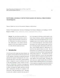
End while After adding the random selection procedure, the time consumption of iteration is greatly reduced. Meanwhile, as the anomalies only have a small probability of occurrence, it is less likely to be chosen in the iteration and therefore is less likely to be learned well. As a result, there is no need to exclude the anomalies before the learning process. It is notable that unlike other over-compete learned dictionaries such as KSVD [41], the elements of the learned dictionary based on random selection can well represent the spectra of major materials and the accurate spectra of materials with a small occupation such as anomalies will not be learned. 3.3. Framework of the Proposed Method The framework of the proposed method is illustrated in Figure 1. The proposed method is based on LRR model and the main idea is to depart the anomaly matrix from the original HSI. For a better and more stable result, a learned dictionary based on sparse coding is adopted to the LRR model. The main steps of the proposed method are described as follows: Step 1: Rearrange the 3-Dimensional hyperspectral image in to a 2-Dimensional matrix X. Step 2: Learn a dictionary D which represents the background spectra from the input HSI data using Algorithm 2. Step 3: By adopting the LRR model and the learned dictionary D, decompose X into a low-rank background matrix L and a sparse anomaly matrix S with inexact ALM using Algorithm 1. Step 4: Apply basic detector on the sparse matrix S to get the detection result. Similar to the RPCA-based AD method [35], the simple and classical GRX method is applied afterwards in our experiments because the proposed method is insensitive to the selection of the basic detector.

Remote Sens. 2016, 8, 289 Remote Sens. 2016, 8, 289

7 of 17 7 of 18

Figure1. 1. Framework Framework of of the the proposed proposedmethod. method. Figure

4. Experiments 4. Experiments and and Discussion Discussion In this this section, section, we we conduct conduct our our experiments experiments on on three threehyperspectral hyperspectralimages, images,one oneof ofwhich whichisisused used In for simulated experiments to analyze the property of the proposed method, and the other two are for simulated experiments to analyze the property of the proposed method, and the other two are used for for real realdata dataexperiment experiment to to demonstrate demonstrate its its effectiveness. effectiveness. It It is is notable notable that that these these three three data data sets sets used are obtained after preprocessing such as atmospheric correlation, and widely used for hyperspectral are obtained after preprocessing such as atmospheric correlation, and widely used for hyperspectral ADproblem. problem. Two-Dimensional Two-Dimensional display display of of the thedetection detectionresult, result,the thereceiver receiveroperating operatingcharacteristic characteristic AD (ROC) [42] and the area under ROC curves (AUC) are the main criteria to evaluate the detection (ROC) [42] and the area under ROC curves (AUC) are the main criteria to evaluate the detection results. results. 4.1. Synthetic Data Experiments 4.1. Synthetic Data Experiments Synthetic data experiments are conducted in this subsection. The effect of parameter choices on Synthetic data experiments areproposed conducted in thisissubsection. The effect parameter on simulated experiment results of the method analyzed. We will thenofcompare thechoices proposed simulated experiment results of method the proposed method is analyzed. Weand will then compare the LRRaLD with the benchmark GRX [8], the state-of-the-art CRD [28], other detectors based proposed LRRaLD with benchmark method [8],[38] thetostate-of-the-art CRD [28], and other on LRMD including RPCAthe [35], LRaSMD GRX [36] and LRASR illustrate its efficiency. detectors based on LRMD including RPCA [35], LRaSMD [36] and LRASR [38] to illustrate its 4.1.1. Synthetic Data Description efficiency. A hyperspectral image, acquired by the HyMap airborne hyperspectral imaging sensor [43] is 4.1.1. Synthetic Data Description used in this subsection. The image data set, covering one area of Cooke City, MT, USA, was collected on 4 JulyA2006, with the spatial size of 200 ˆby 800 and 126 spectral bands spanning the wavelength interval hyperspectral image, acquired the HyMap airborne hyperspectral imaging sensor [43] is of 400–2500 The spectral channels the wavelengths 1320–1410 andUSA, 1800–1980 nm are used in this nm. subsection. The image dataaround set, covering one area of of Cooke City, MT, was collected the and have been in this Eachspanning pixel hasthe approximately on water-absorption 4 July 2006, with bands the spatial size of 200ignored × 800 and 126experiment. spectral bands wavelength 3interval m of ground resolution. Seven types channels of target,around including fabric panel targets andand three vehicle of 400–2500 nm. The spectral thefour wavelengths of 1320–1410 1800–1980 targets, deployed in the region interest of them, shown in TableEach 1, arepixel usedhas as nm are were the water-absorption bands of and have and beenthree ignored in this experiment. buried anomalies simulated experiments. shows spectra of anomalies andpanel background approximately 3 in m our of ground resolution. SevenFigure types2of target, including four fabric targets samples. is notable thatwere among them, F1 andregion F2 areoffull size pixels and of V1them, is a subpixel to and threeItvehicle targets, deployed in the interest and three shown indue Table the ground resolution. Two sub-images of size 150 ˆ 150 are Figure cropped as depicted square 1, are used as buried anomalies in our simulated experiments. 2 shows spectrainofred anomalies frames in Figure 3.samples. One sub-image has a that relatively simple another hasand a complex and background It is notable among them,background F1 and F2 and are full size one pixels V1 is a background. the proposed method is evaluated of background. subpixel dueEffectiveness to the groundofresolution. Two sub-images of size on 150these × 150two are kinds cropped as depicted in red square frames in Figure 3. One sub-image has a relatively simple background and another one Table background. 1. Characteristics of the implanted spectramethod in our synthetic data experiments. has a complex Effectiveness of thetarget proposed is evaluated on these two kinds of background. Name

Type

F1 redspectra cottonin our synthetic data experiments. Table 1. Characteristics of the implanted target F2 yellow nylon Name Type V1 1993 Chevy Blazer

F1 red cotton F2 yellow nylon In the following simulated experiments, to better approach the real environment, 25 random V1 1993 Chevy Blazer locations with different abundance fractions f (ranging from 0.04 to 1) of the specific anomaly spectrum t are buried in the background pixel with spectrum b on both two sub-images respectively, as shown In the following simulated experiments, to better approach the real environment, 25 random locations with different abundance fractions f (ranging from 0.04 to 1) of the specific anomaly spectrum t are buried in the background pixel with spectrum b on both two sub-images respectively,

Remote Sens. 2016, 8, 289 Remote Sens. 2016, 8, 289 Remote Sens. 2016, 8, 289 Remote Sens. 2016, 8, 289

8 of 17 8 of 18 8 of 18 8 of 18

shown inas Figure 4a,b as an example. Figure 4c is the corresponding ground truth. Simple linear in as Figure 4a,b an example. Figure 4c is the corresponding ground truth. Simple linear mixed model as shown in Figure 4a,b as an example. Figure 4c is the corresponding ground truth. Simple linear mixed model is adopted for the buried pixels using the following formula: is adopted for the buried pixels using the following formula: as shown in Figure 4a,b for as an Figure 4c isthe thefollowing corresponding ground truth. Simple linear mixed model is adopted theexample. buried pixels using formula: mixed model is adopted for the buried pixels formula: z = using f ⋅ t + the (1 − following f )⋅b (12) (12) z “z = f ¨ ft ⋅`t +p1(1´− ffq)¨⋅bb (12) z = f ⋅ t + (1 − f ) ⋅ b (12)

Reflectance Reflectance Reflectance

4000 4000 4000

F1 F1 F2 F1 F2 V1 F2 V1 background V1 background background

3000 3000 3000 2000 2000 2000 1000 1000 1000 0 0 500 0 500 500

1000 1000 1000

1500 2000 1500 2000 wavelength/nm 1500 2000 wavelength/nm wavelength/nm Figure 2. Spectra of anomalies and background samples

2500 2500 2500

Figure backgroundsamples samples. Figure2.2.Spectra Spectraof ofanomalies anomalies and and background Figure 2. Spectra of anomalies and background samples

Figure 3. HyMap data set. Figure 3. HyMap data set. Figure data set. set. Figure 3. 3. HyMap HyMap data

(a) (b) (c) (a) (b) (c) (a) with: (a) simple background; (b) (b) complex background; and (c)(c) ground-truth. Figure 4. Sub-images

Figure 4. Sub-images with: (a) simple background; (b) complex background; and (c) ground-truth. Figure 4. Sub-images with: (a) simple background; (b) complex background; and (c) ground-truth. Figure 4. Sub-images 4.1.2. Parameter Analysiswith: (a) simple background; (b) complex background; and (c) ground-truth.

4.1.2. Parameter Analysis 4.1.2.The Parameter Analysis initial choices of different parameters are important for many algorithms. For example, in 4.1.2. Parameter The initialAnalysis choices of different parameters are important for many algorithms. For example, in the CRD method, different sizes of windows areare needed to achieve optimal results for different data The method, initial choices of different parameters important for many algorithms. For example, in the CRD different sizes of windows are needed to achieve optimal results for different data The initial choices of different parameters are important for many algorithms. For example, in sets. The method, rank of the low-rank matrix and theare level of sparsity are required in the LRaSMD method, the CRD different sizes of windows needed to achieve optimal results for different data sets. The rank of the low-rank matrix and the level of sparsity are required in the LRaSMD method, thein CRD method, sizes of parameters windows needed to achieve optimal results for the different data which the best setting of these are often difficult torequired grasp. In the tradeoff sets. The rank ofdifferent the low-rank matrix and theare level of sparsity theRPCA, LRaSMD in which the best setting of these parameters are often difficultare to grasp. Ininthe RPCA, the method, tradeoff sets. The rank of the low-rank matrix and the level of sparsity are required in the LRaSMD method, parameter creates a balance between the low-rank matrix and the sparse matrix, and is crucial to the in which the best setting of between these parameters are often difficult grasp.matrix, In the and RPCA, the tradeoff parameter creates a balance the low-rank matrix and thetosparse is crucial to the the decomposition algorithm. the LRASR, the tradeoff parameter andthe a sparse in successfulness which the creates bestofsetting of these parameters areInoften difficult to grasp. In theand RPCA, tradeoff parameter a balance between the low-rank matrix and the sparse matrix, is crucial to the successfulness of the decomposition algorithm. In the LRASR, the tradeoff parameter and a sparse constrain of theofalow-rank representation matrixIn ismatrix required. the proposed method, the tradeoff parameter creates balance between the low-rank andInthe sparse matrix, and isand crucial to the successfulness the decomposition algorithm. the LRASR, the tradeoff parameter a sparse constrain of the low-rank representation matrix is required. In the proposed method, the tradeoff parameter λ and thedecomposition number N of elements of theIn learned dictionary are also important. successfulness of the algorithm. the LRASR, the tradeoff parameter and a sparse constrain of the low-rank representation matrix is required. In the proposed method, the tradeoff parameter λ and the number N of elements of the learned dictionary are also important. constrain of the low-rank representation matrix required. In the are proposed method, the tradeoff parameter λ and the number N of elements of theislearned dictionary also important. parameter λ and the number N of elements of the learned dictionary are also important.

Remote Sens. 2016, 8, 289 Remote RemoteSens. Sens.2016, 2016,8,8,289 289

9 of 17 99of of18 18

11

11

0.95 0.95

0.95 0.95

0.9 0.9 0.85 0.85

AUC AUC

11 0.95 0.95 AUC AUC

AUC AUC

To To evaluate evaluate the the robustness robustness of of the the proposed proposed LRRaLD LRRaLD method method to to its its parameters, parameters, the the AUCs AUCs are are calculated under different λ using spectra of calculated under different λ and N with two synthetic data sets, using spectra of F1, F2 and V1 calculated under different λ and N with two synthetic data sets, using spectra of F1, F2 and V1 as as Figures 5 5and 6. 6. Experiments areare repeated 20 times to reduce the anomalies, respectively, as shown Figures repeated 20 to anomalies,respectively, respectively,as asshown showninin in Figures 5 and and 6. Experiments Experiments are repeated 20 times times to reduce reduce the acquired by positions to results the As in effect acquired by random positions to obtain results of theof average AUC.AUC. As shown in Figures 5 and 565 theeffect effect acquired byrandom random positions toobtain obtain results of theaverage average AUC. Asshown shown inFigures Figures and 6, the average AUC formed with these two parameters represents a flat surface-like shape, all the average AUC formed with these two parameters represents a flat surface-like shape, all except and 6, the average AUC formed with these two parameters represents a flat surface-like shape,for all except for Figure isis the anomaly of artificially introduced car on Figure thewhich anomaly spectrum ofspectrum an artificially introduced on complex except 6c, forwhich Figureis6c, 6c, which the anomaly spectrum of an an artificiallycar introduced carbackground. on complex complex background. may aa result caused by of cars This may be This aThis result caused by similar of spectra other cars originated from the background. mayofbe beinterference result of of interference interference caused spectra by similar similar spectra of other other cars originated originated from background. ItIt can seen 6c complicated background. It can also be seen frombe Figure that Figure for the complex background, the from the the complicated complicated background. can also also be seen6cfrom from Figure 6c that that for for the the complex complex background, the result isis better when N as aa because larger This more detection result is detection better when N is set as a larger number. This more background information background, the detection result better when N isis set set as is larger number. number. This isis because because more background information can learned the background when isis large. under can be learned in the complex background N is large. Even under suchN results are background information can be be learned in inwhen the complex complex background when Nconditions, large. Even Even under such results are satisfactory, confirmed by >> 0.9. This experiment the satisfactory, confirmed AUC > 0.9. This experiment illustrates robustness of illustrates the proposed such conditions, conditions, resultsby are satisfactory, confirmed by AUC AUC 0.9.the This experiment illustrates the robustness of proposed method in aspects: (1) dictionary, even at size, method in two aspects: (1) the learned dictionary, at alearned small size, contains enough spectra of robustness of the the proposed method in two two aspects:even (1) the the learned dictionary, even at aa small small size, contains enough spectra of background to enable the acquisition of satisfactory experimental results; background to enable the acquisition of satisfactory experimental results; and (2) the proposed method contains enough spectra of background to enable the acquisition of satisfactory experimental results; and (2) method isis robust is robust to proposed the tradeoff parameter λ. to and (2) the the proposed method robust tothe thetradeoff tradeoffparameter parameterλ. λ.

0.9 0.9 0.85 0.85

0.8 0.8 10 10 55 λλ

00 10 10

20 20

30 30 NN

40 40

0.8 0.8 10 10

50 50

0.9 0.9 0.85 0.85

55 λλ

(a) (a)

00 10 10

20 20

30 30 NN

40 40

0.8 0.8 10 10

50 50

55 λλ

(b) (b)

00 10 10

20 20

30 30 NN

40 40

50 50

(c) (c)

Figure 5. AUC surfaces the detection Figure 5. 5. The The AUC AUCsurfaces surfaces of of the thedetection detection results results of of LRRaLD LRRaLD with with different different parameters parameters (λ (λ and and N) N) Figure The of results of LRRaLD with different parameters (λ and N) under simple background: (a) F1; (b) F2; and (c) V1. under simple background: (a) F1; (b) F2; and (c) V1. under simple background: (a) F1; (b) F2; and (c) V1.

0.9 0.9

0.85 0.85

AUC AUC

11 0.95 0.95

AUC AUC

11 0.95 0.95

AUC AUC

11 0.95 0.95

0.9 0.9

0.85 0.85

0.8 0.8 10 10 55 λλ

00 10 10

(a) (a)

20 20

30 30 NN

40 40

50 50

0.9 0.9

0.85 0.85

0.8 0.8 10 10 55 λλ

00 10 10

(b) (b)

20 20

30 30 NN

40 40

50 50

0.8 0.8 10 10 55 λλ

00 10 10

20 20

30 30 NN

40 40

50 50

(c) (c)

Figure Figure 6. 6. The The AUC AUC surfaces surfaces of of the the detection detection results results of of LRRaLD LRRaLD with with different different parameters parameters (λ (λ and and N) N) Figure 6. The AUC surfaces of the detection results of LRRaLD with different parameters (λ and N) under complex background: (a) F1; (b) F2; and (c) V1. under complex background: (a) F1; (b) F2; and (c) V1. under complex background: (a) F1; (b) F2; and (c) V1.

To To better better illustrate illustrate the the effectiveness effectiveness of of LD, LD, we we fix fix N N of of LD LD at at 30 30 and and compare compare the the result result of of LRR LRR To better illustrate the effectiveness of LD, we data fix N of LD atas30the and compare the resultthe of LRR using using usingdifferent differentdictionaries: dictionaries:(1) (1)LD; LD;(2) (2)the thewhole whole datamatrix matrix as thedictionary; dictionary;and and(3) (3) thedictionary dictionary different dictionaries: (1) LD; (2) the in whole data matrix as the dictionary; and (3) the dictionary used used used in in [38]. [38]. The The dictionary dictionary used used in [38] [38] isis constructed constructed with with the the k-means k-means method method and and aims aims at at in [38]. The dictionary used in [38] is constructed with the k-means method and aims at representing representing representing the the background background spectra. spectra. With With the the recommended recommended setting setting as as [38], [38], 300 300 samples samples from from the the the background spectra. With the recommended setting as [38], 300 samples from the image are chosen image image are are chosen chosen to to construct construct the the background background dictionary. dictionary. The The AUCs AUCs using using these these dictionaries dictionaries under under to construct the background dictionary. The AUCs using these dictionaries under different λ are shown different λ are shown in Figures 7 and 8. The original LRR method uses the whole matrix different λ are shown in Figures 7 and 8. The original LRR method uses the whole matrix as as its its in Figures 7 and 8. The original LRR method uses the whole matrix as its dictionary, in which a large λ dictionary, dictionary,in inwhich which aa large largeλλcauses causesaa larger largerrank rank for forthe the low-rank low-rankmatrix, matrix, while while aa small smallλλresults resultsin in causes a larger rank for the low-rank matrix, while a small λ results in a larger sparsity level for the aa larger larger sparsity sparsity level level for for the the sparse sparse matrix, matrix, both both of of which which enables enables possible possible degrade degrade of of detection detection sparse matrix, both of which enables possible degrade of detection results. This is due to the fact that results. results. This This isis due due to to the the fact fact that that its its dictionary dictionary includes includes the the spectra spectra of of anomalies. anomalies. As As aa result, result, the the its dictionary includes is the spectra of anomalies. As a result, the original LRR method is sensitive when to the original original LRR LRR method method is sensitive sensitive to to the the tradeoff tradeoff parameter parameter λ. λ. With With regards regards to to the the anomalies, anomalies, when tradeoff parameter λ. With regards to the anomalies, when adoptingand LD, which mainly represents the adopting adopting LD, LD, which which mainly mainly represents represents the the spectra spectra of of background background and mitigates mitigates the the contamination contamination spectra of background and mitigates the contamination problem, large residuals can still be preserved problem, problem, large large residuals residuals can can still still be be preserved preserved in in the the sparse sparse matrix. matrix. Better Better results results are are obtained obtained with with in theusing sparse matrix. Better results are obtained[38]. with LRRmay using because LD than LRR using the dictionary LRR LRR usingLD LDthan thanLRR LRRusing usingthe thedictionary dictionaryin in [38].This This maybe be becausethe thebackground backgroundspectra spectraof of higher accuracy are obtained through the learning procedure. Two different trends of LRR using LD higher accuracy are obtained through the learning procedure. Two different trends of LRR using LD

the contrary, the spectrum of V1, as shown in Figure 2, is the spectrum of a subpixel, which makes its the contrary, the spectrum of V1, as shown in Figure 2, is the spectrum of a subpixel, which makes its spectrum harder to obtain in the learning process. As a result, more stable result is obtained when spectrum harder to obtain in the learning process. As a result, more stable result is obtained when using V1 as anomalies. Overall, the results in Figures 7 and 8 show that LRR using LD is more robust using V1 as anomalies. Overall, the results in Figures 7 and 8 show that LRR using LD is more robust and has a better performance. and has a better performance. Meanwhile, given that LD is of small size, less computation of the LRMD procedure 10 of ofthe Remote Sens. 2016, 8, 289 17 Meanwhile, given that LD is of small size, less computation of the LRMD procedure of the proposed method is required compared to the original LRR method. Under an 8-core Intel Xeon proposed method is required compared to the original LRR method. Under an 8-core Intel Xeon E5504 with 24 GB of DDR3 RAM, it costs 26.08 s for the proposed method and 88.34 s for the original E5504 with 24 GB of DDR3 RAM, it costs 26.08 s for the proposed method and 88.34 s for the original in [38]. This in may because the background spectra of higher accuracy are obtained throughonthe LRR method thebe decomposition and the basic GRX procedures when using F1 as anomalies a LRR method in the decomposition and the basic GRX procedures when using F1 as anomalies on a learning procedure. Two different trends of LRR using LD as dictionary can be viewed in Figure simple background. However, an additional computation of learning process is required for 7a,c. the simple background. However, an additional computation of learning process is required for the This is might because whenthe using F1calculation and F2 as anomalies, notmatlab totally proposed method, in which main is obtainingthe thecontamination sparse vectors.problem By usingisthe proposed method, in which the main calculation is obtaining the sparse vectors. By using the matlab eliminated for LD as well as the dictionary used in [38]. On the contrary, the spectrum of V1, as shown toolbox spams [44], the computational time is greatly reduced, costing 10.87 s to learn a dictionary. toolbox spams [44], the computational time is greatly reduced, costing 10.87 s to learn a dictionary. in Figure is the spectrum a subpixel, makes its spectrum harder obtain the learning The total 2, execution time ofofthe proposedwhich method is 36.95 s, still far less tothan theinoriginal LRR The total execution time of the proposed method is 36.95 s, still far less than the original LRR process. As a result, more stable result is obtained when using V1 as anomalies. Overall, the results in method. In later experiments, λ is fixed at 1 and N is fixed at 30 for the proposed LRRaLD method. method. In later experiments, λ is fixed at 1 and N is fixed at 30 for the proposed LRRaLD method. Figures 7 and 8 show that LRR using LD is more robust and has a better performance. The execution time of the learning process is also included for the proposed method. The execution time of the learning process is also included for the proposed method. 1 1

0.9 0.9 AUC AUC

0.6 0.6 0.5 0 0.5

0.9 0.9

0.8 0.8

0.8 0.8

0.7 0.7

0.7 0.7

0

LRR using LD as dictionary LRR using LDas asdictionary dictionary LRR using itself LRR using as dictionary LRR using theitself dictonary in [38] LRR using the dictonary in [38] 2 4 6 8 10 2 4λ 6 8 10

1

0.9 0.9 AUC AUC

0.8 0.8

1

1

AUC AUC

1

0.6 0.6 0.5 0 0.5

0

λ

(a) (a)

LRR using LD as dictionary LRR using LD as dictionary LRR using itself as dictionary LRR using itself asindictionary LRR using dictionary [38] LRR using dictionary in [38] 2 4 6 8 10 2 4 6 8 10

λ

0.7 0.7 0.6 0.6 0.5 0 0.5

λ

(b) (b)

0

LRR using LD as dictionary LRR using LDas asdictionary dictionary LRR using itself LRR using as dictionary LRR using theitself dictonary in [38] LRR using the dictonary in [38] 2 4 6 8 10 2 4 6 8 10

λ

(c) (c)

λ

Figure 7. AUC with different tradeoff parameter λλ under simple background using different Figure Figure7.7. AUC AUC with with different different tradeoff tradeoff parameter parameter λ under under simple simple background background using using different different dictionaries: (a) F1; (b) F2; and (c) V1. dictionaries: dictionaries:(a) (a)F1; F1;(b) (b)F2; F2;and and(c) (c)V1. V1. 1

1

1

1

1

1

0.8 0.8

0.8 0.8

0.8 0.8

0.7 0.7 0.6 0.6 0.5 0 0.5

0


λ

λ

(a) (a)

AUC AUC

0.9 0.9

AUC AUC

0.9 0.9

AUC AUC

0.9 0.9

0.7 0.7 0.6 0.6 0.5 0 0.5

0


λ

λ

(b) (b)

0.7 0.7 0.6 0.6 0.5 0 0.5

0

LRR using LD as dictionary LRR using LDas asdictionary dictionary LRR using itself LRR using itself asindictionary LRR using dictionary [38] LRR using dictionary in [38] 2 4 6 8 10 2 4 6 8 10

λ

λ

(c) (c)

Figure 8. AUC with different tradeoff parameter λ under complex background using different Figure 8. AUC with different tradeoff parameter λ under complex background using different Figure 8. AUC with different parameter λ under complex background using different dictionaries: (a) F1; (b) F2; and (c)tradeoff V1. dictionaries: (a) F1; (b) F2; and (c) V1. dictionaries: (a) F1; (b) F2; and (c) V1.

4.1.3. Detection Performance 4.1.3. Detection Performance Meanwhile, given that LD is of small size, less computation of the LRMD procedure of the In this subsection, we compare the proposed method with GRX, CRD, RPCA, LRaSMD and In this subsection, we compared compare the proposed with GRX, RPCA, and proposed method is required to the originalmethod LRR method. UnderCRD, an 8-core IntelLRaSMD Xeon E5504 LRASR. The spectra of F1, F2 and V1 are used as spectra of anomalies for the simulated experiment LRASR. The spectra of F1, F2 and V1 are used as spectra of anomalies for the simulated experiment with 24 GB of DDR3 RAM, it costs 26.08 s for the proposed method and 88.34 s for the original LRR respectively. The optimal parameters used for other methods are as follows. For the CRD method, respectively. optimal parameters usedGRX for other methods areusing as follows. For the CRD method in the The decomposition and the basic procedures when F1 as anomalies on amethod, simple we set the size of the inner window at 11 × 11 and the size of the outer window at 15 × 15. For the we set the size of the inner window at 11 × 11 and the size of the outer window at 15 × 15. For the background. However, an additional computation of learning process is required for the proposed LRaSMD method, we set the rank of the low-rank matrix at 8 and the sparsity level at 0.3. For the LRaSMD method, we set the rank of the low-rank matrix at 8 and the sparsity level at 0.3. For the method, in which the main calculation is obtaining the sparse vectors. By using the matlab toolbox RPCA method, different tradeoff parameters are tried and the optimal results are chosen for RPCA[44], method, different tradeoff are tried and10.87 the soptimal are chosen for spams the computational time isparameters greatly reduced, costing to learn results a dictionary. The total different situations due to the sensitivity of the algorithm. For the LRASR method, the sparse different situations due to the sensitivity of the algorithm. For the LRASR method, the sparse execution time of the proposed method is 36.95 s, still far less than the original LRR method. In later constrain of the low-rank representation matrix is set at 0.1, and the tradeoff parameter is set at 10 for constrain of λ the matrix setproposed at 0.1, andLRRaLD the tradeoff parameter is set at 10 for experiments, is low-rank fixed at 1 representation and N is fixed at 30 foristhe method. The execution time the simple background and 0.1 for the complex background for its best performance. background for the for complex background for its best performance. ofthe thesimple learning process isand also0.1 included the proposed method. The 2-Dimensional display of the detection results and its binary result of simple and complex The 2-Dimensional display of the detection results and its binary result of simple and complex backgrounds with F1 randomly implanted as an example are shown in Figures 9 and 10, 4.1.3. Detection Performance backgrounds with F1 randomly implanted as an example are shown in Figures 9 and 10, In this subsection, we compare the proposed method with GRX, CRD, RPCA, LRaSMD and LRASR. The spectra of F1, F2 and V1 are used as spectra of anomalies for the simulated experiment respectively. The optimal parameters used for other methods are as follows. For the CRD method, we set the size of the inner window at 11 ˆ 11 and the size of the outer window at 15 ˆ 15. For the LRaSMD method, we set the rank of the low-rank matrix at 8 and the sparsity level at 0.3. For the RPCA method, different tradeoff parameters are tried and the optimal results are chosen for different


11 of 17

situations due to the sensitivity of the algorithm. For the LRASR method, the sparse constrain of the low-rank representation matrix is set at 0.1, and the tradeoff parameter is set at 10 for the simple background and 0.1 for the complex background for its best performance. The 2-Dimensional display of the detection results and its binary result of simple and complex backgrounds with F1 randomly implanted as an example are shown in Figures 9 and 10 respectively. The binary results are obtained with the probability of false alarm rate (PFA) equals 10´3 . The more pixels detected in the binary display of detection result, the better. The corresponding 11 ROC curves Remote Sens. 2016, 8, 289 of 18 are shown inSens. Figures 11 and 12 respectively. As shown, the proposed LRRaLD method11 detects the Remote 2016, 8, 289 of 18 respectively. The binary results are obtained with ofcurve. false alarm (PFA) equals most anomalies among the five methods. It also hasthe theprobability best ROC CRDrate and LRASR have the −3. The more 10 pixels detected in the result, the better. The respectively. The binary results are binary obtained with of thedetection probability of false alarm ratecorresponding (PFA) following performance both on simple and display complex backgrounds. That might be the equals result of the ROC curves arepixels shown in Figures 11 binary and 12,display respectively. As shown, LRRaLD method 10−3. The more detected in the of detection result,the theproposed better. The corresponding ability of CRD to exploit local information, and LRASR also exploits the structure information of HSI. detects the most anomalies among methods. It As also has the ROC LRRaLD curve. CRD and ROC curves are shown in Figures 11 the and five 12, respectively. shown, thebest proposed method On the contrary, the results of RPCA and are poor thethecomplex background used LRASR have the following performance both methods. on simple complex backgrounds. That CRD might be in the detects the most anomalies among theLRaSMD five Itand alsoon has best ROC curve. and synthetic data experiments. Table 2 shows the average detection rates of 20 repeated experiments the result of the of CRD to exploitboth localon information, LRASR also exploitsThat the structure LRASR have theability following performance simple andand complex backgrounds. might be information of the contrary, the results of RPCA the and LRaSMD are poor on theusing complex the equals result of0.01. theHSI. ability of CRD to exploit local information, andaverage LRASR also exploits the structure when PFA ForOnthe proposed LRRaLD method, detection rate spectrum in the synthetic databackground, experiments. 2 and shows the average detection rates of 20 pixels information of HSI. On the contrary, the results of Table RPCA LRaSMD are on the complex of F1 asbackground anomalies used is 0.946 under simple which means only onepoor or two anomalous repeated experiments PFAdata equals 0.01. For Table the proposed LRRaLD the average background used in thewhen synthetic experiments. 2 shows the averagemethod, rates of 20 are missed. The anomalies with anomalous fraction higher than 0.1 can be welldetection detected. The proposed detection using spectrum of F1equals as anomalies is 0.946 under simple background, means repeated rate experiments when PFA 0.01. For the proposed LRRaLD method,which the average LRRaLDonly hasone theorhighest detection rates and LRASR has the second performance. RPCA and LRaSMD two anomalous pixels Theisanomalies with anomalous fractionwhich higher than detection rate using spectrum of F1are asmissed. anomalies 0.946 under simple background, means have poor results on complex background, which might be because their models are drawn 0.1 beor well Thepixels proposed LRRaLDThe hasanomalies the highest detection rates fraction and LRASR hasthan the from onlycan one twodetected. anomalous are missed. with anomalous higher a singlesecond subspace and cannot handle a complex background. CRD has results onthe complex performance. RPCA and LRaSMD have poor results on complex background, whichhas might 0.1 can be well detected. The proposed LRRaLD has the highest detection ratesgood and LRASR be because their be models are drawn from a poor single subspace and cannot handle alargest complex second performance. RPCA andit LRaSMD have results on complex background, might background. This may because utilizes local information. However, it has thewhich variances CRD has good results on complex background. Thisand may be because it utilizes local be because their models drawn from single subspace handle a complex among background. these five methods dueare to the effect of arandom locations. Incannot general, the results using the information. it hasresults the largest variances among these five methods due to the effect of background. However, CRD has good on complex background. This may be because it utilizes local spectra of F1 and F2 as anomalies are better than the results using the spectrum of V1 as anomalies. random locations. In general, the spectra F1 and F2methods as anomalies arethe better than information. However, it has the theresults largestusing variances amongofthese five due to effect of This may be because spectra of of V1 F1asand F2 are spectra spectra of full pixels and can bebetter better detected the results using the the anomalies. may theanomalies spectra ofare F1 and F2than are random locations. Inspectrum general, the results using the This ofbe F1because and F2 as comparespectra toresults theofspectrum of sub-pixel full pixels can beofbetter compare to the of sub-pixel the using the and spectrum V1V1. asdetected anomalies. This may bespectrum because the spectra ofV1. F1 and F2 are spectra of full pixels and can be better detected compare to the spectrum of sub-pixel V1. LRRaLD GRX CRD RPCA LRaSMD LRASR LRRaLD GRX CRD RPCA LRaSMD LRASR

LRRaLD LRRaLD

GRX GRX

CRD CRD

RPCA RPCA

LRaSMD LRaSMD

LRASR LRASR

Figure 9. Detection results under simple background using different methods: (top) 2-D display; and

Figure 9. Detection results under simple background using different methods: (top) 2-D display; and (bottom) results when PFA equals 0.001. Figure 9. binary Detection results under simple background using different methods: (top) 2-D display; and (bottom) binary results when PFA equals 0.001. (bottom) binary results when PFA equals 0.001. LRRaLD LRRaLD

GRX GRX

CRD CRD

RPCA RPCA

LRaSMD LRaSMD

LRASR LRASR

LRRaLD LRRaLD

GRX GRX

CRD CRD

RPCA RPCA

LRaSMD LRaSMD

LRASR LRASR

Figure 10. Detection results under complex background using different methods: (top) 2-D display; and (bottom) binary results equals 0.001. Figure 10. Detection results when underPFA complex background using different methods: (top) 2-D display;

Figure 10. Detection results under complex background using different methods: (top) 2-D display; and (bottom) binary results when PFA equals 0.001. and (bottom) binary results when PFA equals 0.001.

12 of 17 12 12 of of 18 18 1 1

1 1

0.8 0.8

0.8 0.8

0.8 0.8

0.6 0.6

LRRaLD LRRaLD GRX GRX CRD CRD RPCA RPCA LRaSMD LRaSMD LRASR LRASR

0.4 0.4 0.2 0.2 0 0 -4 10 -4 10

-3

-2

-1

10 -3 10 -2 10 -1 10 10 10 False Alarm Rate False Alarm Rate

0.6 0.6


0.4 0.4 0.2 0.2 0 0 -4 10 -4 10

0

10 0 10

DetectionRate Rate Detection

1 1



Remote Sens. 2016, 8, 289 Remote Remote Sens. Sens. 2016, 2016, 8, 8, 289 289

-3

-2

-1


0.4 0.4 0.2 0.2 0 0 -4 10 -4 10

0


(a) (a)

0.6 0.6

10 0 10

-3

-2

-1


(b) (b)

0

10 0 10

(c) (c)

1 1

1 1

0.8 0.8

0.8 0.8

0.8 0.8

0.6 0.6


0.4 0.4 0.2 0.2 0 0 -4 10 -4 10

-3

-2

-1


0

10 0 10

0.6 0.6


0.4 0.4 0.2 0.2 0 0 -4 10 -4 10


1 1



Figure 11. ROC curves under simple background using different methods: (a) F1; (b) F2; and (c) V1. Figure ROC curves under simple background using different methods: and Figure 11.11. ROC curves under simple background using different methods: (a)(a) F1;F1; (b)(b) F2;F2; and (c)(c) V1.V1.

-3

-2

-1


0.4 0.4 0.2 0.2

0


(a) (a)

0.6 0.6

10 0 10

(b) (b)

0 0 -4 10 -4 10

-3

-2

-1


0

10 0 10

(c) (c)

Figure Figure 12. 12. ROC ROC curves curves under under complex complex background background using using different different methods: methods: (a) (a) F1; F1; (b) (b) F2; F2; and and (c) (c) V1. V1. Figure 12. ROC curves under complex background using different methods: (a) F1; (b) F2; and (c) V1. Table Table 2. 2. Average Average detection detection rates rates when when PFA PFA equals equals 0.01 0.01 (20 (20 repetitions). repetitions). Table 2. Average detection rates when PFA equals 0.01 (20 repetitions). Simple Different Simple Background Background Different Methods F1 F2 V1 Methods F1 Simple Background F2 V1 Different 0.946 ± 0.027 0.906 ± 0.047 0.816 ± 0.057 LRRaLD Methods 0.946 ± 0.027 0.906 0.816 LRRaLD F1 F2 ± 0.047 V1 ± 0.057 GRX 0.682 0.644 0.522 GRX 0.682 ±± 0.009 0.009 0.644 ±± 0.012 0.012 0.522 ±± 0.020 0.020 LRRaLD CRD 0.946 ˘ 0.027 0.9060.846 ˘ 0.047 0.816 ˘ 0.057 0.866 0.776 CRD 0.866 ±± 0.072 0.072 0.846 ±± 0.086 0.086 0.776 ±± 0.079 0.079 GRX RPCA0.682 ˘ 0.009 0.644 ˘ 0.012 0.522 ˘ 0.020 0.930 ±± 0.018 ±± 0.020 0.456 ±± 0.027 RPCA0.866 ˘ 0.930 0.0180.8460.864 0.864 0.020 0.776 0.456 0.027 CRD LRaSMD 0.072 ˘ 0.086 ˘ 0.079 0.852 ±± 0.029 0.790 ±± 0.069 0.530 ±± 0.045 LRaSMD 0.852 0.029 0.790 0.069 0.530 0.045 RPCA LRASR0.930 ˘ 0.018 0.864 ˘ 0.020 0.456 ˘ 0.027 0.870 ±± 0.018 0.828 ±± 0.019 0.792 ±± 0.016 LRASR 0.870 0.018 0.828 0.019 0.792 0.016 LRaSMD 0.852 ˘ 0.029 0.790 ˘ 0.069 0.530 ˘ 0.045 LRASR 0.870 ˘ 0.018 0.828 ˘ 0.019 0.792 ˘ 0.016

Complex Complex Background Background F1 ComplexF2 Background V1 F1 F2 V1 0.800 ± 0.067 0.762 0.826 ± 0.058 0.800 ±F2 0.067 0.762 ±± 0.073 0.073 0.826F1± 0.058 V1 0.518 0.510 0.478 0.518 ±± 0.028 0.028 0.510 ±± 0.022 0.022 0.478 ±± 0.042 0.042 0.826 ˘ 0.058 0.800 ˘ 0.067 0.742 0.762 ˘ 0.073 0.798 0.778 0.798 ±± 0.072 0.072 0.778 ±± 0.081 0.081 0.742 ±± 0.098 0.098 0.518 ˘± 0.028 0.510±˘0.121 0.022 0.384 0.478 ˘ 0.042 0.594 0.144 0.572 ±± 0.077 0.594 ± 0.144 0.572 ± 0.121 0.384 0.077 0.798 ˘ 0.072 0.778 ˘ 0.081 0.742 ˘ 0.098 0.630 0.119 0.552 ± 0.048 0.424 ±± 0.132 0.630˘±± 0.144 0.119 0.552 0.048 0.424 0.132 0.594 0.572±±˘0.044 0.121 0.748 0.384 ˘ 0.077 0.842 ± 0.024 0.758 ± 0.048 0.842˘± 0.119 0.024 0.758 ± 0.048 0.630 0.552±˘0.044 0.048 0.748 0.424 ˘ 0.132 0.842 ˘ 0.024 0.758 ˘ 0.044 0.748 ˘ 0.048

Table Table 33 is is the the execution execution time time of of the the different different methods. methods. The The proposed proposed method method has has aa less less execution time than CRD, in which the inverse function of local background requires heavy execution time than CRD, in which the inverse function of local background requires heavy Table 3 is the execution time of the different methods. The proposed method has a less execution computational cost. It also notable that RPCA is C which might its computational It is is notable that the the RPCA is run run with withrequires C code, code,heavy whichcomputational might accelerate accelerate time than CRD, incost. which thealso inverse function of local background cost.its efficiency. efficiency. It is also notable that the RPCA is run with C code, which might accelerate its efficiency. Table 3. time of different methods on synthetic data sets (20 repetitions). Table 3. Execution Execution time different methods synthetic data repetitions). Table 3. Execution time of of different methods onon synthetic data setssets (20(20 repetitions). Time(s) LRRaLD GRX CRD RPCA LRaSMD LRASR Time(s) LRRaLD GRX CRD RPCA LRaSMD LRASR Time(s) GRX CRD±± 0.70 RPCA LRASR Simple background 40.46 5.37 42.39 16.68 36.03 355.5 Simple background LRRaLD 40.46 ±± 0.20 0.20 5.37 ±± 0.16 0.16 42.39 0.70 16.68 ±± 0.27 0.27 LRaSMD 36.03 ±± 0.40 0.40 355.5 ±± 21.5 21.5 Complex background 41.28 ±± 0.46 ±± 0.33 42.48 ±± 1.10 18.29 ±± 0.23 35.98 ± 0.51 376.2 ± 18.5 Complex background 40.46 41.28 0.46 5.375.40 5.40 0.33 42.39 42.48 1.10 16.68 18.29 0.23 36.03 35.98 0.51 355.5 376.2 18.5 Simple background ˘ 0.20 ˘ 0.16 ˘ 0.70 ˘ 0.27 ˘ ±0.40 ˘±21.5

Complex background

41.28 ˘ 0.46

5.40 ˘ 0.33

42.48 ˘ 1.10

18.29 ˘ 0.23

35.98 ˘ 0.51

376.2 ˘ 18.5

4.2. 4.2. Real Real Data Data Experiments Experiments 4.2. Real Data Experiments In In this this section, section, two two widely widely used used real real HSI HSI data data sets, sets, which which contain contain ground-truth, ground-truth, are are applied applied to to evaluate the performance of the proposed method. GRX, CRD, RPCA, LRaSMD and LRASR are In this the section, two widely usedproposed real HSI data sets,GRX, whichCRD, contain ground-truth, evaluate performance of the method. RPCA, LRaSMD are andapplied LRASRtoare used comparisons. evaluate performance of the proposed method. GRX, CRD, RPCA, LRaSMD and LRASR are used used as asthe comparisons. as comparisons. 4.2.1. 4.2.1. Real Real Data Data Sets Sets Description Description 4.2.1. Real Data Sets Description One One real real data data set set was was acquired acquired by by the the Hyperion Hyperion imaging imaging sensor sensor [45], [45], which which has has 242 242 bands bands with with aa spectral resolution of 10 nm over 357–2576 nm. The image data set was collected in 2008, covering One real data set was acquired by the Hyperion imaging sensor [45], which has 242 bands spectral resolution of 10 nm over 357–2576 nm. The image data set was collected in 2008, covering an area State Indiana, USA. After of bands the with spectral resolution of 10 nm of over 357–2576 nm. Theremoval image data setlow-SNR was collected 2008, an aagricultural agricultural area of of the the State of Indiana, USA. After removal of the the low-SNR bandsinand and the uncalibrated bands, 149 bands are used. The 150 × 150 sub-image with the ground truth of the covering an agricultural area of the State of Indiana, USA. After removal of the low-SNR bands and uncalibrated bands, 149 bands are used. The 150 × 150 sub-image with the ground truth of the anomalies anomalies is is used. used. Where Where the the anomalies anomalies come come from from the the storage storage silo silo and and the the roof, roof, these these anomalies, anomalies,


13 of 17

the uncalibrated bands, 149 bands are used. The 150 ˆ 150 sub-image with the ground truth of the Remote Sens. 2016, 8, 289 13 of 18 Remote Sens. 2016, 8, 289 13 of 18 anomalies is used. Where the anomalies come from the storage silo and the roof, these anomalies, especially the storage silo, areare not visually distinguishable fromthe the background. The scene and the especially the storage not from the background. The scene and especially the storagesilo, silo,are notvisually visually distinguishable distinguishable from background. The scene and thethe ground truth of anomalies are shown in Figure 13. ground truth of anomalies are shown in Figure 13. ground truth of anomalies are shown in Figure 13.

(a) (a)

(b)

(b)

Figure 13. Hyperion data set: (a) RGB composite (36, 23, 12); and (b) ground-truth.

Figure 13.13.Hyperion (36,23, 23,12); 12);and and(b) (b)ground-truth. ground-truth. Figure Hyperiondata dataset: set: (a) (a) RGB RGB composite composite (36,

The other one was collected by HYDICE airborne sensor and can be downloaded from the

The otherone onewas wascollected collected by HYDICE HYDICE airborne airborne sensor be from the The other sensor and andcan canThe bedownloaded downloaded from website of the Army GeoSpatial by Center (www.agc.army.mil/hypercube/). spatial resolution is the website of the Army GeoSpatial Center (www.agc.army.mil/hypercube/). The spatial resolution is approximately 1 m, and the whole data(www.agc.army.mil/hypercube/). set has a size of 307 × 307. However, only upperresolution right of website of the Army GeoSpatial Center Thethe spatial is approximately 1 am, and the datawhich set has a size of 307 × 307. onlyinthe upper of the scene with size 80 whole ×whole 100 pixels, with redHowever, square frame 14a,right has approximately 1 m, andofthe data set hasisadisplayed size of 307 ˆ a307. However, onlyFigure the upper right of theascene with a sizetruth of 80for × 100 pixels, which isThis displayed with red square framefor inhyperspectral Figure 14a, has definite anomaly cropped areaaawas the scene withground a size of 80 ˆ 100 pixels,detection. which is displayed with redwidely squareused frame in Figure 14a, has a definite ground truth for anomaly detection. This cropped area was widely used for hyperspectral anomaly detection [28,45] and is utilized for our real data experiment. Here, 175 bands remain after a definite ground truth for anomaly detection. This cropped area was widely used for hyperspectral anomaly detection [28,45] andabsorption is utilized bands. for our There real data Here,21175anomalous bands remain after removal of water vapor areexperiment. approximately pixels, anomaly detection [28,45] and is utilized for our real data experiment. Here, 175 bands remain after removal of water vapor absorption bands. There are approximately 21 anomalous pixels, representing cars and roof. The scene and its corresponding ground-truth map of anomalies are removal of watercars vapor approximatelyground-truth 21 anomalousmap pixels, cars representing andabsorption roof. Thebands. scene There and itsarecorresponding of representing anomalies are illustrated in Figure 14b,c. and roof. Theinscene and its corresponding ground-truth map of anomalies are illustrated in Figure 14b,c. illustrated Figure 14b,c.

(a)

(b)

(c)

Figure 14.(a) HYDICE data set: (a) RGB composite (b)(55, 31, 22); (b) region of interest; and (c) (c)ground-truth.

Figure 14. HYDICE data set: (a) RGB composite (55, 31, 22); (b) region of interest; and (c) ground-truth. 4.2.2. Detection Performance Figure 14. HYDICE data set: (a) RGB composite (55, 31, 22); (b) region of interest; and (c) ground-truth.

In this subsection, we compare the proposed method with GRX, CRD, RPCA, LRaSMD and 4.2.2. Detection Performance 4.2.2.LRASR Detection Performance on real data sets. As mentioned in Section 4.1.2, we fix the tradeoff parameter λ at 1 and the In thisNsubsection, compare method with GRX, RPCA, data LRaSMD and number of elements we of LD at 30 forthe theproposed proposed LRRaLD method. On CRD, the Hyperion set, the In this subsection, weAs compare theinproposed method with tradeoff GRX, CRD, RPCA,λ LRaSMD and LRASR on parameters real data sets. mentioned Section we For fix the parameter at 1size andofthe optimal used for other methods are as4.1.2, follows. the CRD method, we set the LRASR on real data sets. As mentioned in Section 4.1.2, we fix the tradeoff parameter λ at 1 and number N of elements of×LD at 30the forsize theofproposed LRRaLDatmethod. On the theLRaSMD Hyperionmethod, data set, the inner window at 11 11 and the outer window 15 × 15. For wethethe number N of elements of LD at 30 for the proposed LRRaLD method. On the Hyperion data set,ofthe set theparameters rank of theused low-rank matrix at 8 and at 0.3. Formethod, the RPCA the optimal for other methods arethe as sparsity follows.level For the CRD we method, set the size optimal parameters used other methods as follows. For CRD method, the size parameter is set 0.02.the For theof LRASR method, we set ofwe theset low-rank thetradeoff inner window at 11 × for 11atand size theare outer window at the 15the ×sparse 15. Forconstrain the LRaSMD method, we of theset inner window at 11 ˆ 11 and the size of the outer window at 15 ˆ 15. For the LRaSMD method, representation 0.1 and the tradeoff parameter at 5. On the HYDICE urban data set, the optimal the rank of the low-rank matrix at 8 and the sparsity level at 0.3. For the RPCA method, the parameters for other methods areatas For thewe CRD method, weFor set the the size the inner the wetradeoff set the parameter rank used of the matrix 8follows. and the sparsity level 0.3. RPCA method, islow-rank set at 0.02. For the LRASR method, set theat sparse constrain ofofthe low-rank window at 7 × 7 and the size of the outer window at 15 × 15, the same optimal parameters as used in tradeoff parameter at the 0.02.tradeoff For theparameter LRASR method, the sparse constrain theoptimal low-rank representation at is 0.1set and at 5. Onwe theset HYDICE urban data set,ofthe [28]. For the RPCA method, the tradeoff parameter is set at 0.015. For the LRaSMD and LRASR parameters used forand other methods are as follows.atFor method, we set the size the optimal inner representation at 0.1 the tradeoff parameter 5. the On CRD the HYDICE urban data set,ofthe methods, same settings as the Hyperion data set are adopted. window atused 7 × 7for andother the size of the outer 15 ×the 15,CRD the same optimal in parameters methods are aswindow follows.atFor method, we parameters set the size as of used the inner Figures 15 and 16 are the detection results of Hyperion data set and HYDICE data set, [28]. For method, parameter is set at the 0.015. For optimal the LRaSMD and LRASR window at 7the ˆ RPCA 7 and the size ofthe thetradeoff outer window at 15 ˆ 15, same parameters as used respectively, Figure 17 is the corresponding ROC curves, and Table 4 illustrates the AUC and settings as the Hyperion dataparameter set are adopted. in methods, [28]. For same thetime RPCA method, the tradeoff is set at 0.015.outperforms For the LRaSMD and LRASR execution of different methods. The proposed LRRaLD method other methods. Figures 15 and 16 are the detection results of Hyperion data set and HYDICE data set, methods, same settings as the Hyperion data set are adopted. respectively, Figure 17 is the corresponding ROC curves, and Table 4 illustrates the AUC and execution time of different methods. The proposed LRRaLD method outperforms other methods.


14 of 17

Figures 15 and 16 are the detection results of Hyperion data set and HYDICE data set, respectively, Figure 17 is the corresponding ROC curves, and Table 4 illustrates the AUC and execution time of different methods. The proposed LRRaLD method outperforms other methods. When using the Remote Sens. 2016, 8, 289 14 of Remote Sens. 2016, 8, 289 1418 of 18 HYDICE data set, the proposed method has alike performance as other methods at the low FAR Remote Sens. 2016, 8, 289 14 of 18 area. When This isusing mainly because theset, stripped noises of the HYDICE data setasas have amethods relatively When HYDICE data set, theproposed proposed method has alike other at at high using thethe HYDICE data the method has alikeperformance performance other methods low FAR area. Thisisis mainly because the method strippedhas noises the data setset have a a magnitude. The LRMD methods can the stripped noises from the original image. However, When using the HYDICE data set, separate the proposed alike of performance as other methods at thethe low FAR area. This mainly because the stripped noises of theHYDICE HYDICE data have relatively high magnitude. The LRMD methods can separate the stripped noises from the original the low FAR area. This is mainly because the stripped noises of the HYDICE data set have a the information of noise will remain in the sparse matrix, which makes the FAR high and affect the relatively high magnitude. The LRMD methods can separate the stripped noises from the original image. However, the information of noise will remain in the sparse matrix,noises whichfrom makes the FAR relatively high magnitude. The LRMD methods can separate the stripped the original image. However, the information of statistic noise will in the sparsefor matrix, which makes the FAR detection results. Figure 18 shows the ofremain detection values the AD algorithm. Each group high and affect the detection results. Figure 18 shows in thethe statistic detection values forthe theFAR AD image. However, information of noise will sparseofmatrix, which makes and affect the the detection results. Figure 18 remain shows the statistic of detection values for the AD box. has ahigh green box representing the anomalous pixels and a blue box representing the background algorithm. Eachthe group has aresults. green Figure box representing anomalous pixelsvalues and aforblue high and affect detection 18 shows thethe statistic of detection the box AD algorithm. Eachedges group has box a green boxand representing the anomalous pixelsThe and a blue LRRaLD box The upper and low of the are 10th respectively. representing the background The90th upper and lowpercentiles, edgesthe of the box are 90th andand 10thproposed algorithm. Each group has box. a green box representing anomalous pixels apercentiles, blue box representing the background box. The upper and low edges of the box are 90th and 10th percentiles, methodrespectively. has the best performance. The proposed LRRaLD method performance. representing the background box. The upper has andthe lowbest edges of the box are 90th and 10th percentiles, respectively. The proposed LRRaLD method has the best performance.

respectively. The proposed LRRaLD method has the best performance. LRRaLD GRX CRD RPCA LRaSMD LRRaLD GRX CRD RPCA LRaSMD LRRaLD GRX CRD RPCA LRaSMD

LRRaLD

GRX

CRD

LRRaLD LRRaLD

GRX GRX

CRD CRD

RPCA RPCA RPCA

LRaSMD LRaSMD LRaSMD

LRASR LRASR LRASR

LRASR LRASR LRASR

Figure 15. Detection results of Hyperion data set: (top) 2-D display; and (bottom) binary results

Figure 15. Detection results of Hyperion data set: (top) 2-D display; and (bottom) binary results when when 0.001. FigurePFA 15. equals Detection results of Hyperion data set: (top) 2-D display; and (bottom) binary results Figure 0.001. 15. Detection results of Hyperion data set: (top) 2-D display; and (bottom) binary results PFA equals when PFA equals 0.001. when PFA equals 0.001.

LRRaLD LRRaLD

GRX GRX

LRRaLD

GRX

LRRaLD LRRaLD

GRX GRX

LRRaLD

GRX

CRD CRD

RPCA RPCA

LRaSMD LRaSMD

LRASR LRASR

CRD CRD

RPCA RPCA

LRaSMD LRaSMD

LRASR LRASR

CRD

RPCA

CRD

RPCA

LRaSMD

LRASR

LRaSMD

LRASR

Figure 16. Detection results of HYDICE data set: (top) 2-D display; and (bottom) binary results when PFA equals 0.001. results of HYDICE data set: (top) 2-D display; and (bottom) binary results when Figure 16. Detection

1 0.8

1 0.8

0.8 0.6

0.8 0.6

1

LRRaLD GRX LRRaLD CRD GRX RPCA LRRaLD CRD LRaSMD GRX RPCA LRASR CRD LRaSMD

Detection Rate

0.8

0.6 0.4

0.60.4 0.2

0.40.2 0 -4 0.2 10 0 -4 10

0 -4 10

RPCA LRASR -2 -1 0 10 10 10 LRaSMD -2 -1 0 False Alarm Rate 10 10 10LRASR 10 False (a)Alarm Rate -3

10

-3

-3

Detection Detection Detection Rate RateRate

Detection Detection RateRate

Figure 16. Detection results of HYDICE data set: (top) 2-D display; and (bottom) binary results when PFA 16. equals 0.001. results of HYDICE data set: (top) 2-D display; and (bottom) binary results when Figure Detection 1 1 0.001. PFA equals PFA equals 0.001. 1 LRRaLD GRX LRRaLD CRD GRX RPCA LRRaLD CRD LRaSMD GRX RPCA LRASR CRD LRaSMD

0.8

0.6 0.4

0.6

0.4 0.2

0.4 0.2 0 -4 10 0.2 0 -4 10 0

-4

RPCA 0 LRASR -2 -1 10 10 10 LRaSMD0 -2 Rate -1 Alarm 10 10 10 LRASR10 False Alarm Rate (b) -3

10

-3 False

-3

-2

-1

0

-2 -1 0 10 10 10 10 (b) 10 10 10 10 (a) Figure 17. The ROC curves of the AD algorithms for the real data sets: (a) Hyperion data set; and (b)

10

False Alarm Rate

False Alarm Rate

HYDICE Figure 17.data Theset. ROC curves of the AD algorithms for the real data sets: (a) Hyperion data set; and (b) (b) (a) HYDICE data set.

Figure 17. The ROC curves of the AD algorithms for the real data sets: (a) Hyperion data set; and (b)

Figure 17. The ROC curves of the AD algorithms for the real data sets: (a) Hyperion data set; and HYDICE data set. (b) HYDICE data set.

Remote Sens. 2016, 8, 289 Remote Sens. 2016, 8, 289

15 of 17 15 of 18

(a)

(b)

Figure 18. Statistical separability analysis of the AD algorithms: (a) Hyperion data set; and (b) Figure 18. Statistical separability analysis of the AD algorithms: (a) Hyperion data set; and (b) HYDICE HYDICE data set. data set. Table 4. AUC AUC and and execution execution time time of of different different methods. methods. Table 4.

Different Data Sets LRRaLD GRX LRRaLD GRX 0.9998 AUC 0.9978 Hyperion AUC 0.9998 0.9978 Time(s) 41.25 5.90 Hyperion Time(s) 41.25 5.90 0.9988 AUC 0.9872 HYDICE AUC Time(s) 0.9988 18.14 0.9872 0.87 HYDICE Different Data Sets

Time(s)

18.14

0.87

CRD 0.9992 0.9992 48.73 48.73 0.9961 0.9961 33.23 CRD

33.23

RPCA LRaSMD LRASR RPCA LRaSMD LRASR 0.9902 0.9981 0.9993 0.9902 0.9981 0.9993 21.91 42.51 336.5 21.91 42.51 336.5 0.9793 0.8918 0.9874 0.9793 0.8918 0.9874 6.53 18.81 140.5 6.53

18.81

140.5

Both experiments on synthetic and real data sets illustrate the advantage of the proposed Both experiments on syntheticthe and real dataLRRaLD sets illustrate the features advantage the proposed LRRaLD LRRaLD method. To summarize, proposed method as of follows: method. To summarize, the proposed LRRaLD method features as follows: 1) Effectiveness: based on LRR, the intrinsic low-rank property of HSI can be well exploited. based LRR, the the intrinsic property of HSI can be well exploited. 1) Compared Effectiveness: to other ADon algorithms, modellow-rank of LRR fits the LMM model better, resulting in a Compared to other higher detection rate.AD algorithms, the model of LRR fits the LMM model better, resulting in a higher detection 2) Robustness: using rate. LD as the dictionary of LRR algorithm, a better separation of anomaly and be LD achieved, which makes the proposed robustoftoanomaly the tradeoff 2) background Robustness:can using as the dictionary of LRR algorithm,method a bettermore separation and parameter as can a result. The experimental results that the proposed is more robust background be achieved, which makes theshow proposed method moremethod robust to the tradeoff to its parameters. parameter as a result. The experimental results show that the proposed method is more robust to 3) Efficiency: with the small size of LD, less computation cost is required, making the procedure its parameters. LRR much faster efficient. experimental showmaking that thethe computational 3) of Efficiency: with the and smallmore size of LD, lessThe computation cost results is required, procedure of cost of the proposed method is in a reasonable range. LRR much faster and more efficient. The experimental results show that the computational cost of the proposed method is in a reasonable range. 5. Conclusions 5. Conclusions In this study, a new anomaly detector based on LRR and LD for hyperspectral imagery is proposed. intrinsic low-rank property of on hyperspectral is exploited using the LRR In this The study, a new anomaly detector based LRR and LD imagery for hyperspectral imagery is proposed. decomposition method.property Meanwhile, a dictionary imagery learning is method is adopted toLRR achieve a relatively The intrinsic low-rank of hyperspectral exploited using the decomposition pure background dictionary, which makes the LRR decomposition procedure both more robust to method. Meanwhile, a dictionary learning method is adopted to achieve a relatively pure background the tradeoffwhich parameter cost decomposition less computation time. Finally, the basic is usedparameter to obtain dictionary, makesand the LRR procedure both more robustdetector to the tradeoff the detection result. and cost less computation time. Finally, the basic detector is used to obtain the detection result. It is is demonstrated demonstrated in the experiments experiments of simulated and data that that the the proposed proposed method method has has It in the of simulated and real real data excellent performance. excellent performance. However, However, the the model model of of LRR LRR only only considers considers anomalies anomalies with with large large magnitude. magnitude. The influence of Gaussian noise should also be considered, which will be the focus of our future The influence of Gaussian noise should also be considered, which will be the focus of our future work. work. Acknowledgments: The authors would like to thank the State Key Laboratory of Information Engineering in Acknowledgments: The authors would like to thank the State Key Laboratory of Information Engineering in Surveying, Mapping Mappingand andRemote Remote Sensing, Wuhan University for providing the Hyperion data set, the Surveying, Sensing, Wuhan University for providing the Hyperion data set, and theand Digital Digital Imaging and Sensing Remote Group, SensingCenter Group, forScience, ImagingRochester Science, Rochester of Technology for Imaging and Remote forCenter Imaging Institute ofInstitute Technology for the HyMap data set used in our experiments. The authorsThe would also would like to thank Zebin Wu from Nanjing University the HyMap data set used in our experiments. authors also like to thank Zebinthe Wu from the Nanjing of Science and Technology for sharingfor thesharing code ofthe LRASR, and the anonymous reviewers for the insightful University of Science and Technology code of LRASR, and the anonymous reviewers for the comments and suggestions. This research was supported by the National Natural Science Foundation of China insightful comments and suggestions. This research was supported by the National Natural Science Foundation (Grant No. 61572133), and the Research fund for the State Key Laboratory of Earth Surface Processes and Resource of Chinaunder (GrantGrant No. 61572133), and the Research fund for the State Key Laboratory of Earth Surface Processes Ecology 2015-KF-01. and Resource Ecology under Grant 2015-KF-01.


16 of 17

Author Contributions: Yubin Niu mainly was responsible for modeling, experiments designing, and manuscript writing. Bin Wang gave the research idea and insightful suggestions to the manuscript. Conflicts of Interest: The authors declare no conflict of interest.

References 1. 2. 3. 4. 5.

6. 7.

8. 9. 10. 11. 12. 13.

14. 15. 16.

17. 18. 19. 20. 21. 22.

Shaw, G.; Manolakis, D. Signal processing for hyperspectral image exploitation. IEEE Signal Process. Mag. 2002, 19, 12–16. [CrossRef] Chang, C.I.; Chiang, S. Anomaly detection and classification for hyperspectral imagery. IEEE Trans. Geosci. Remote Sens. 2002, 40, 1314–1325. [CrossRef] Shaw, G.; Manolakis, D. Detection algorithm for hyperspectral imaging application. IEEE Signal Process. Mag. 2002, 19, 29–43. Manolakis, D.; Lockwood, R.; Cooley, T.; Jacobson, J. Is there a best hyperspectral detection algorithm? Proc. SPIE 2009, 7334, 1–17. [CrossRef] Jin, S.; Wang, B. A preprocessing method based on independent component analysis with references for target detection in hyperspectral imagery. In Proceedings of the Audio, Language and Image Processing (ICALIP), Shanghai, China, 7–9 July 2014; pp. 537–542. Nasrabadi, N.M. Hyperspectral Target Detection: An overview of current and future challenges. IEEE Signal Process. Mag. 2014, 31, 34–44. [CrossRef] Ben Salem, M.; Ettabaa, K.S.; Hamdi, M.A. Anomaly detection in hyperspectral imagery: An overview. In Proceedings of the Image Processing, Applications and Systems Conference (IPAS), Sfax, Tunisia, 5–7 November 2014; pp. 1–6. Reed, I.S.; Yu, X. Adaptive multiple-band CFAR detection of an optical pattern with unknown spectral distribution. IEEE Trans. Acoust. Speech Signal Process. 1990, 38, 1760–1770. [CrossRef] Nasrabadi, N.M. Regularization for spectral matched filter and RX anomaly detector. Proc. SPIE 2008, 6966, 1–12. Matteoli, S.; Diani, M.; Corsini, G. Improved estimation of local background covariance matrix for anomaly detection in hyperspectral images. Opt. Eng. 2010, 49, 046201. [CrossRef] Heesung, K.; Nasrabadi, N.M. Kernel RX-algorithm: A nonlinear anomaly detector for hyperspectral imagery. IEEE Trans. Geosci. Remote Sens. 2005, 43, 388–397. [CrossRef] Gu, Y.; Liu, Y.; Zhang, Y. A selective KPCA algorithm based on high-order statistics for anomaly detection in hyperspectral imagery. IEEE Geosci. Remote Sens. Lett. 2008, 1, 43–47. [CrossRef] Guo, Q.; Zhang, B.; Ran, Q.; Gao, L.; Li, J.; Plaza, A. Weighted-RXD and linear filter-based RXD: Improving background statistics estimation for anomaly detection in hyperspectral imagery. IEEE J. Sel. Top. Appl. Earth Observ. Remote Sens. 2014, 7, 2351–2366. [CrossRef] Du, B.; Zhang, L. Random-selection-based anomaly detector for hyperspectral imagery. IEEE Trans. Geosci. Remote Sens. 2010, 49, 1578–1589. [CrossRef] Wang, L.; Chang, C.I. Multiple-window anomaly detection for hyperspectral imagery. IEEE J. Sel. Top. Appl. Earth Observ. Remote Sens. 2008, 6, 644–658. Liu, W.; Chang, C.I. A nested spatial window-based approach to target detection for hyperspectral imagery. In Proceedings of the IEEE International Geoscience and Remote Sensing Symposium (IGARSS), Anchorage, AK, USA, 20–24 September 2004; Volume 1, pp. 20–24. Khazai, S.; Safari, A.; Mojaradi, B.; Homayouni, S. An approach for subpixel anomaly detection in hyperspectral images. IEEE J. Sel. Top. Appl. Earth Observ. Remote Sens. 2013, 6, 769–778. [CrossRef] Chang, C.I.; Heinz, D.C. Constrained subpixel target detection for remotely sensed imagery. IEEE Trans. Geosci. Remote Sens. 2000, 38, 1144–1159. [CrossRef] Carlotto, M.J. A cluster-based approach for detecting man-made objects and changes in imagery. IEEE Trans. Geosci. Remote Sens. 2005, 43, 374–387. [CrossRef] Banerjee, A.; Burlina, P.; Diehl, C. A support vector method for anomaly detection in hyperspectral imagery. IEEE Trans. Geosci. Remote Sens. 2006, 44, 2282–2291. [CrossRef] Sakla, W.; Chan, A.; Ji, J.; Sakla, A. An SVDD-based algorithm for target detection in hyperspectral imagery. IEEE Geosci. Remote Sens. Lett. 2011, 8, 384–388. [CrossRef] Yuan, Y.; Ma, D.; Wang, Q. Hyperspectral anomaly detection by graph pixel selection. IEEE Trans. Cybern. 2015, 1–12. [CrossRef] [PubMed]


23. 24. 25. 26. 27. 28. 29. 30. 31. 32. 33.

34. 35. 36. 37. 38. 39. 40.

41. 42. 43.

44. 45.

17 of 17

Yuan, Y.; Wang, Q.; Zhu, G. Fast hyperspectral anomaly detection via high-order 2-D crossing filter. IEEE Trans. Geosci. Remote Sens. 2015, 2, 620–630. [CrossRef] Ranney, K.I.; Soumekh, M. Hyperspectral anomaly detection within the signal subspace. IEEE Geosci. Remote Sens. Lett. 2006, 3, 312–316. [CrossRef] Chen, Y.; Nasrabadi, N.M.; Tran, T.D. Hyperspectral image classification using dictionary-based sparse representation. IEEE Trans. Geosci. Remote Sens. 2011, 49, 3973–3985. [CrossRef] Chen, Y.; Nasrabadi, N.M.; Tran, T.D. Hyperspectral image classification via kernel sparse representation. IEEE Trans. Geosci. Remote Sens. 2013, 51, 217–231. [CrossRef] Chen, Y.; Nasrabadi, N.M.; Tran, T.D. Sparse representation for target detection in hyperspectral imagery. IEEE J. Sel. Top. Signal Process. 2011, 5, 629–640. [CrossRef] Li, W.; Du, Q. Collaborative representation for hyperspectral anomaly detection. IEEE Trans. Geosci. Remote Sens. 2015, 53, 1463–1474. [CrossRef] Li, J.; Zhang, H.; Zhang, L.; Ma, L. Hyperspectral anomaly detection by the use of background joint sparse representation. IEEE J. Sel. Top. Appl. Earth Observ. Remote Sens. 2015, 8, 2523–2533. [CrossRef] Niu, Y.; Wang, B. Hyperspectral target detection using learned dictionary. IEEE Geosci. Remote Sens. Lett. 2015, 12, 1531–1535. Candès, E.J.; Li, X.; Ma, Y.; Wright, J. Robust principal component analysis? J. ACM 2011, 58, 1–37. [CrossRef] Zhao, Y.; Yang, J. Hyperspectral image denoising via sparse representation and low-rank constraint. IEEE Trans. Geosci. Remote Sens. 2015, 53, 296–308. [CrossRef] Zhou, T.; Tao, D. Godec: Randomized low-rank & sparse matrix decomposition in noisy case. In Proceedings of the 28th International Conference on Machine Learning (ICML), Bellevue, WA, USA, 28 June–2 July 2011; pp. 33–40. Zhang, H.; He, W.; Zhang, L.; Shen, H.; Yuan, Q. Hyperspectral image restoration using low-rank matrix recovery. IEEE Trans. Geosci. Remote Sens. 2014, 52, 4729–4743. [CrossRef] Chen, S.; Yang, S.; Kalpakis, K.; Chang, C.I. Low-rank decomposition-based anomaly detection. Proc. SPIE 2013, 8743, 1–7. Sun, W.; Liu, C.; Li, J.; Lai, Y.M.; Li, W. Low-rank and sparse matrix decomposition-based anomaly detection for hyperspectral imagery. J. Appl. Remote Sens. 2014, 8, 1–18. [CrossRef] Liu, G.; Lin, Z.; Yan, S.; Sun, J.; Yu, Y.; Ma, Y. Robust recovery of subspace structures by low-rank representation. IEEE Trans. Pattern Anal. Mach. Intell. 2013, 35, 171–184. [CrossRef] [PubMed] Xu, Y.; Wu, Z.; Li, J.; Plaza, A.; Wei, Z. Anomaly detection in hyperspectral images based on low-rank and sparse representation. IEEE Trans. Geosci. Remote Sens. 2016, 54, 1990–2000. [CrossRef] Charles, A.S.; Olshausen, B.A.; Rozell, C.J. Learning sparse codes for hyperspectral imagery. IEEE J. Sel. Top. Signal Process. 2011, 5, 963–978. [CrossRef] Charles, A.S.; Olshausen, B.A.; Rozell, C.J. Sparse coding for spectral signatures in hyperspectral images. In Proceeding of the 44th Asilomar Conference on Signals, Systems and Computers (ASILOMAR), Pacific Grove, CA, USA, 7–10 November 2010; pp. 191–195. Aharon, M.; Elad, M.; Bruckstein, A. K-SVD: An algorithm for designing overcomplete dictionaries for sparse representation. IEEE Trans. Signal Process. 2006, 54, 4311–4322. [CrossRef] Kerekes, J. Receiver operating characteristic curve confidence intervals and regions. IEEE Geosci. Remote Sens. Lett. 2008, 5, 251–255. [CrossRef] Snyder, D.; Kerekes, J.; Fairweather, I.; Crabtree, R.; Shive, J.; Hager, S. Development of a web-based application to evaluate target finding algorithms. In Proceedings of the IEEE International Geoscience and Remote Sensing Symposium (IGARSS), Boston, MA, USA, 7–11 July 2008; Volume 2, pp. 915–918. Mairal, J.; Bach, F.; Ponce, J.; Sapiro, G. Online learning for matrix factorization and sparse coding. J. Mach. Learn. Res. 2010, 11, 19–60. Du, B.; Zhang, L. A discriminative metric learning based anomaly detection method. IEEE Trans. Geosci. Remote Sens. 2014, 11, 6844–6857. © 2016 by the authors; licensee MDPI, Basel, Switzerland. This article is an open access article distributed under the terms and conditions of the Creative Commons by Attribution (CC-BY) license (http://creativecommons.org/licenses/by/4.0/).

Hyperspectral Anomaly Detection Based on Low-Rank ... - MDPI

Hyperspectral Anomaly Detection Based on Low-Rank ... - MDPI

Suggest Documents

Hyperspectral Anomaly Detection Based on Low-Rank ... - MDPI

Kernel-Based Anomaly Detection in Hyperspectral

HYPERSPECTRAL ANOMALY DETECTION IN URBAN SCENARIOS

hyperspectral anomaly detection: a comparative ... - Semantic Scholar

HYPERSPECTRAL ANOMALY DETECTION IN URBAN SCENARIOS

Structured Background Modeling for Hyperspectral Anomaly Detection

Anomaly detection and classification for hyperspectral imagery

Hyperspectral Anomaly Detection: Comparative Evaluation in Scenes

A Robust Nonlinear Hyperspectral Anomaly Detection Approach

Hyperspectral Chemical Plume Detection Algorithms Based On

anomaly-based hyperspectral image compression - CiteSeerX

Hyperspectral Chemical Plume Detection Algorithms Based On

Network-Wide Anomaly Detection Based on

NETWORK ANOMALY DETECTION BASED ON ...

Incremental Anomaly-based Intrusion Detection

Gravitation-Based Edge Detection in Hyperspectral Images - MDPI

Feature-based anomaly detection - CiteSeerX

Graph-Based Anomaly Detection - CiteSeerX

Botnet Detection based on Anomaly and Community Detection - Site BU

An Entropy-Based Network Anomaly Detection Method - MDPI

An Entropy-Based Network Anomaly Detection Method - MDPI

Real-time anomaly detection in hyperspectral images using ...

Hyperspectral Anomaly Detection by the Use of Background Joint ...

Hyperspectral Target Detection via Adaptive Information ... - MDPI