HYPERSPECTRAL IMAGE DATA MINING FOR BAND SELECTION IN AGRICULTURAL APPLICATIONS S. G. Bajwa, P. Bajcsy, P. Groves, L. F. Tian
ABSTRACT. Hyperspectral remote sensing produces large volumes of data, quite often requiring hundreds of megabytes to gigabytes of memory storage for a small geographical area for one−time data collection. Although the high spectral resolution of hyperspectral data is quite useful for capturing and discriminating subtle differences in geospatial characteristics of the target, it contains redundant information at the band level. The objective of this study was to identify those bands that contain the most information needed for characterizing a specific geospatial feature with minimal redundancy. Band selection is performed with both unsupervised and supervised approaches. Five methods (three unsupervised and two supervised) are proposed and compared to identify hyperspectral image bands to characterize soil electrical conductivity and canopy coverage in agricultural fields. The unsupervised approach includes information entropy measure and first and second derivatives along the spectral axis. The supervised approach selects hyperspectral bands based on supplemental ground truth data using principal component analysis (PCA) and artificial neural network (ANN) based models. Each hyperspectral image band was ranked using all five methods. Twenty best bands were selected by each method with the focus on soil and plant canopy characterization in precision agriculture. The results showed that each of these methods may be appropriate for different applications. The entropy measure and PCA were quite useful for selecting bands with the most information content, while derivative methods could be used for identifying absorption features. ANN measure was the most useful in selecting bands specific to a target characteristic with minimum information redundancy. The results also indicated that a combination of wavebands with different bandwidths will allow use of fewer than 20 bands used in this study to represent the information contained in the top 20 bands, thus reducing image data dimensionality and volume considerably. Keywords. Band selection, Data mining, Hyperspectral, Precision agriculture, Remote sensing.
P
recision farming practices are conceptually based on within−field variability information. Modern sensing technologies including remote sensing for information gathering results in large volumes of raw data. Remote sensing can provide high−resolution data on geospatial variability in yield−limiting soil and crop variables. It can be used for mapping soil characteristics (Ahn et al., 1999; Bajwa et al., 2001), leaf area index (LAI), crop development (Ghinelli and Bennet, 1998), canopy coverage, pest infestation, plant water content (Bach and Mauser, 1995), and crop stresses (Gopalapillai and Tian, 1999; Bajwa
Article was submitted for review in June 2003; approved for publication by the Information & Electrical Technologies Division of ASAE in April 2004. The use of trade names, proprietary products, or specific equipment is only meant to provide specific information to the reader, and does not constitute a guarantee or warranty by the University of Arkansas or the University of Illinois and does not imply the approval of the named product to the exclusion of other products that may be suitable. The authors are Sreekala G Bajwa, ASAE Member Engineer, Assistant Professor, Department of Biological and Agricultural Engineering, University of Arkansas, Fayetteville, Arkansas; and Peter Bajcsy, Associate Research Scientist, National Center for Supercomputing Applications, Peter Groves, Graduate Student, Department of Computer Sciences, and Lei F. Tian, ASAE Member Engineer, Associate Professor, Department of Biological and Agricultural Engineering, University of Illinois at Urbana−Champaign, Urbana, Illinois. Corresponding author: Sreekala Bajwa, Assistant Professor, Department of Biological and Agricultural Engineering, University of Arkansas, 203 Engineering Hall, Fayetteville, AR 72701; phone: 479−575−2878; fax: 479−575−2846; e−mail:
[email protected].
and Tian, 2001). Lack of data mining tools and inability of agriculture producers and consultants to extract useful information from large volumes of raw data on yield−limiting factors is a major hurdle in the widespread application of remote sensing at production level. The benefits of hyperspectral sensors come from relatively high spatial and spectral resolutions (Birk and McCord, 1994). The high spectral resolution aids in discovering subtle differences in narrow−band reflectance caused by different vegetation and soil characteristics that are not discernible with multispectral data. However, much of the information in hyperspectral data is redundant. Individual hyperspectral bands are spatially and spectrally correlated (fig. 1). Removal of redundancy and identification of the most significant hyperspectral bands for characterizing a specific geospatial phenomenon is of utmost interest to several application domains. Most of the commercially available remote sensing algorithms and software packages were developed for multispectral data processing, mainly for commercially available image data (Karimi, 1998). There are not many analytical tools developed for hyperspectral data processing. The analytical tools developed for multispectral data fail to make use of added information in hyperspectral data (Schowengerdt, 1997). Although high dimensionality in hyperspectral images results in increased class separability in classification problems, it leads to high errors in parameter estimation (Hsieh and Landgrebe, 1998a). There is ongoing research to modify parametric classification methods to fully utilize added information in hyperspectral data without the loss of accuracy in parameter
Transactions of the ASAE Vol. 47(3): 895−907
E 2004 American Society of Agricultural Engineers ISSN 0001−2351
895
0.01 0.008
0.6
0.006
0.4
0.004
0.2
0.002
0 −0.2470
520
570
620
670
720
770
−0.4
−0.004
−0.6 −0.8
0 820 −0.002 −0.006
Correlation
Variance
Covariance
−1
Variance, Covariance
Inter−Correlation of bands
1 0.8
−0.008 −0.01
Wavelength (nm)
Figure 1. Interrelationship between image bands of a hyperspectral image. Correlation and covariance of band 1 with respect to all 120 bands, and band 1 variance, are plotted against band wavelength for field 2.
estimation (Hsieh and Landgrebe, 1998b; Tu, 2000). An alternate method that would extract information pertinent to one or more target properties without assuming a data distribution would be of great interest to applications in precision agriculture, forestry, and environmental monitoring. The concept of signature bands or bands that are most responsive to a specific target characteristics is similar to the spectral fingerprints used in geological and mining applications (Schowengerdt, 1997). Unlike the space−scale aspect of spectral fingerprints, the signature bands utilize the absorbance−reflectance characteristics of individual wavebands or waveband regions. The experimental application of hyperspectral data in precision farming is focused on mapping narrow−band target reflectance to ground measurements used for crop characterizations. Signature band identification will be useful not only for geospatial characterization of specific target properties but also for application−dependent hyperspectral data compression and sensor characterization. Our goal is to evaluate five methods for band selection from hyperspectral data with or without knowledge of the application domain. Signature bands can be extracted by using two fundamental approaches: unsupervised and supervised. The unsupervised approaches are application independent. They include information entropy measure and first and second derivatives along the spectral axis. The supervised approaches select hyperspectral bands based on supplemental ground data using principal component analysis (PCA) and an artificial neural network (ANN) based model. We focus on methods for hyperspectral band selection that lead to data compression and spectral signature characterization. From a compression standpoint, these methods differ from pixel−based compression techniques such as that defined by the Joint Photographic Expert’s Group (JPEG) (Taubman and Marcellin, 2000). The proposed methods compress data at the band level rather than at the pixel level as done by JPEG (Taubman and Marcellin, 2000). From a spectral signature characterization viewpoint, we propose a variety of methods that are appropriate for representation (information entropy, PCA) or for class discrimination (first and second derivative along spectral axis, ANN). While concise image representation and class discrimination methods have different objectives, a tradeoff of both objectives can provide satisfactory compression and classification results for an application. For example, an orthogonal subspace projection approach to classify images consider-
896
ably reduced data dimensionality while detecting spectral signatures of interest (Harsanyi and Chang, 1994). Another example would be a statistical separation method based on spatial autocorrelation that optimized the selection of bands with and without a priori knowledge of the scene (Petrie and Heasler, 1998). The three major objectives of our study were to: S Research and develop three unsupervised methods for rank ordering of bands from hyperspectral imagery. The methods are based on evaluation of each band separately with three different criteria. The first method is based on an information entropy criterion. The second and third methods are based on a residual criterion derived from the first and second derivatives along spectral axis with two and three adjacent bands, respectively. S Design and implement two supervised methods based on ANN and PCA that use ground truth data for band selection. S Compare the results obtained from the unsupervised and supervised methods.
METHODOLOGY EXPERIMENTAL DESIGN Remote sensing data were acquired from three agricultural fields located in the Midwest U.S. These three fields included field 1 and field 2 located in Missouri, and field 3 located in Illinois (table 1). Hyperspectral image data were collected from fields 1 and 2 on April 26, 2000, and from field 3 on June 8, 2000. The supplemental ground data for fields 1 and 2 included two measures of apparent soil electrical conductivity (ECa, in mS/m) measured with two different devices. The first device was a Geonics EM−38RT (Geomatrix Earth Science, Ltd., Hockliffe, U.K.), which measured ECa in the top 120 cm of soil using a non−invasive method called electromagnetic (EM) induction. The ECa data collected with the Geonics EM−38RT are referred to as EM data in this article. The second device was a VERIS 3100 soil mapping system, which is a direct−contact soil EC meter. The ECa data collected by the VERIS mapping system are referred to as VERIS data. The VERIS shallow (VERIS−s) represented the ECa for the top 33 cm soil, and the VERIS deep (VERIS−d) represented the ECa for the top 100 cm soil.
TRANSACTIONS OF THE ASAE
Table 1. Descriptions of the three fields used in the study. Field Area (ha) Crop Image Date Field 1, Missouri Field 2, Missouri Field 3, Illinois
36 15 16
Soybean Corn Soybean
April 26, 2000 April 26, 2000 June 8, 2000
The ECa is a good indicator of yield−limiting soil physical and chemical properties such as soil texture, Ca, Mg, K, and CEC in some soils, and soil water content (Fritz et al., 1999; Kitchen et al., 2000). The soil EC measurements have long been used to identify contrasting soil properties in the geological and environmental domains (Lund et al., 1999). The ground data for field 3 included canopy coverage, measured as a fraction of ground area covered by crop canopy. The canopy coverage was measured for every 16 cm square area in the field. The canopy coverage was collected on June 8, 2000, with a vehicle−mounted vision system (Tian et al., 1999). Ground truth data were collected with the objective of characterizing specific geospatial variability within a field at a maximum possible resolution. The resolution of the VERIS and EM data was approximately 10 m between adjacent passes. A summary of the ground truth database used in this study is given in table 2. Both EM and VERIS data showed very high variabilitywithin each field. IMAGE ACQUISITION AND PREPROCESSING The image data were collected from an aerial platform with a NASA RDACS/H−3, 120−channel prism−grating, pushbroom hyperspectral sensor. Each image had 2500 rows, 640 columns, and 120 bands per pixel. The 120 bands corresponded to the visible to near−infrared range of 471 to 828 nm, recorded at a spectral resolution of 3 nm. The hyperspectral sensor was mounted on a fixed−wing aircraft and was flown over the fields for data collection. The images were collected from altitudes of approximately 1200 m and 2250 m. The ground spatial interval (GSI) of the images was approximately 1 m for fields 1 and 2, and 2 m for field 3. The image preprocessing included four steps: (1) image calibration for sensor noise, (2) correction for geometric distortion caused by platform motion, (3) image georegistration, and (4) image calibration for variable illumination (fig. 2). The sensor−based noise varied with weather conditions. On each day of data collection, an image was taken with the lens covered to obtain the noise data for the sensor. This image was called the dark image. To minimize sensor noise, the raw image was first transformed with the help of the dark image into a minimum noise fraction (MNF) image (Green et al., 1988). The MNF transformation is similar to a principal Raw Image
Dark Image Placard Image
MNF Transform
MNF Transform
MNF Transform
Distortion Correction
Table 2. Geographic database of the experimental fields listing the statistics on apparent soil electrical conductivity measurements (ECa) made with EM and VERIS instruments (in mS/m) and canopy coverage as a ratio of canopy area to ground area. Field Variable[a] Field Mean Variance Min. Max.
[a]
Field 1 (Missouri)
ECa−EM ECa−VERIS−s ECa−VERIS−d
30.71 9.74 19.61
14.08 9.89 72.24
15.85 1.60 2.30
77.74 34.70 53.80
Field 2 (Missouri)
ECa−EM ECa−VERIS−s ECa−VERIS−d
34.79 15.21 23.71
40.83 56.74 133.51
0 1.50 2.60
60.33 62.30 77.00
Field 3 (Illinois)
Canopy coverage
0.203
0.017
0
1
EM refers to ECa measured with a Geonics EM38RT, which measures up to 120 cm depth in soil. VERIS−s refers to ECa measured up to 33 cm depth, and VERIS−d refers to ECa measured up to 100 cm depth with VERIS equipment.
component transform. The bands of the MNF image that contained significant information were transformed back to image space using inverse MNF transform. The hyperspectral images acquired with the airborne pushbroom scanner showed varying degrees of geometric distortion caused by platform motion under atmospheric turbulence. Roll, pitch, and yaw of the aircraft led to significant geometric errors in pushbroom scanner data. Among the platform−based errors, the aircraft roll was the major source of image distortion, followed by aircraft pitch. The images after correcting for sensor noise were preprocessed to eliminate platform−based geometric distortion. Figure 3a illustrates image distortion caused by aircraft roll. The image shows gradual shifting of linear features, resulting in a distorted field boundary. To eliminate roll, first a known linear feature along the in−track direction was identified in the image. Then each row of the image was shifted in the cross−track direction to straighten the known linear feature. After correcting the image for geometric error caused by platform roll, the image layout (fig. 3b) appeared closer to the actual field layout. The geometric distortion due to pushbroom scanner geometry was considered negligible because of the low altitude of the airborne sensor (a maximum of 7500 ft) and the small area covered in each image. The distortion−corrected images were then georeferenced using a triangulation method with bilinear resampling (fig. 3). Fifteen to twenty ground control points (GCP) distributed inside and outside the field boundary were used for georeferencing each image. Markers or white−painted boards placed in and around the field along with static features such as pumps, crossroads, and field corners were Crop, Orient
Sensor Noise
Inverse MNF
Geo− reference
Calibrate
Collect Placard Spectra
Inverse MNF
Calibrated Image
Compute Calibration Factors
Figure 2. Flowchart showing the steps in image preprocessing for correction, georeferencing, and calibration (“MNF transform” refers to minimum noise fraction transformation).
Vol. 47(3): 895−907
897
(a)
(b)
Figure 3. A raw image of field 1: (a) platform−based image distortion, and (b) after correcting for error caused by platform roll.
used as GCPs. All the images were corrected and calibrated using ENVI software package (Research Systems, Inc., Boulder, Colo.). The georeferenced images were corrected for variable illumination using an empirical line method (Smith and Milton, 1999). The raw images come as digital numbers (DN) or gray−level values. The empirical line calibration procedure transformed the DNs to apparent reflectance of the target, which does not change significantly with illumination conditions. For applying the empirical line method of calibration, markers or tarps (also called placards) of eight different reflectance levels of 2%, 4%, 8%, 16%, 32%, 48%, 64%, and 83% were placed on the field at the time of imaging. Hyperspectral images of placards were taken at the same resolution as the hyperspectral images of the field on each collection day. The empirical line method assumes that the calibrated values are linearly related to the uncalibrated values. This linear relationship between the known reflectance and the observed DNs of the placards was calculated by linear regression and applied to the whole image. The image acquisition time was limited to between 10:00 a.m. and 2:00 p.m. to minimize the errors due to the changes in sun angle. UNSUPERVISED METHODS FOR BAND SELECTION The three unsupervised methods of hyperspectral band selection did not require image preprocessing since they are application−independent techniques based on spatial and spectral similarity of bands. The two supervised methods (PCA and ANN) required image preprocessing into apparent reflectance since they used a model of target characteristics on hyperspectral data to establish the band order. The first and second derivatives and the ANN methods were implemented in the software environment called Data to Knowledge (D2K) developed under the Image to Knowledge (I2K) tools at the National Center for Supercomputing Applications (NCSA, 2000). Method 1: Information Entropy Information entropy is based on evaluating each band separately using the entropy measure (H) defined in equation 1:
where p is the probability of occurrence of a DN in a hyperspectral band, and m is the number of distinct DNs in that band. The probabilities are estimated by computing a histogram of DNs. Generally, if the entropy value (H) is high, then the amount of information in the data is large. Thus, the bands are ranked in descending order from the band with the highest entropy value (large amount of information) to the band with the smallest entropy value (small amount of information). Method 2: First Spectral Derivative The bandwidth of each band can be a variable in hyperspectral sensor design. The first spectral derivative method explores the bandwidth variable as a function of added information. It is apparent that if two adjacent bands do not differ much, then the underlying geospatial phenomenon can be characterized with only one band. The mathematical description of first spectral derivative is illustrated in equation 2: D1 =
i =1
898
(1)
(2)
where I represents the hyperspectral value, x is a spatial location, and l is the band characteristic or central wavelength. Thus, if D1 is equal to zero, then one of the bands is redundant. In general, adjacent bands that differ a lot should be preserved for characterization, while similar adjacent bands can be reduced. In addition to evaluating band characteristics, this method is instrumental in bandwidth design of a remote hyperspectral sensor. Method 3: Second Spectral Derivative Similar to method 2, the second spectral derivative explores the bandwidth variable in hyperspectral imagery as a function of added information. Contrary to method 2, this approach identifies bands that can be represented by a linear combination of adjacent bands. Thus, if two adjacent bands can linearly interpolate the third band, then the third band is redundant. The larger the deviation from a linear model, the higher the information value of the band. The mathematical description of this method is shown in equation 3:
m
H = − ∑ pi ln pi
∂I (x, λ) ∂λ
D2 =
∂ 2 I (x, λ) ∂λ2
(3)
TRANSACTIONS OF THE ASAE
SUPERVISED METHODS FOR BAND SELECTION Method 4: Artificial Neural Network (ANN) Artificial neural networks are used in a wide variety of applications and in many disciplines because of their robustness in making predictions based on training examples. They are particularly applicable in agricultural problems for modeling complex relationships, where stochastic factors play major roles (Mukherjee, 1997). An example of ANN application in precision agriculture is to model the relationship between yield−limiting factors estimated with remote sensing data and yield measurements (Goh, 1995; Gopalapillai and Tian, 1999). Stochastic factors cause significant spatial variations in crop yield (20% to 80%, according to Bakhsh et al., 1998). Therefore, remote sensing is a valuable tool to monitor the in−season effect of stochastic factors on a near−real−time basis. In order to train the ANN algorithm, training data was converted into ASCII format and then normalized. A plain text file was created with entries containing geographical position, field data (EM, VERIS, and canopy), and the reflectance data from each of the 120 bands of spectral data. Each column of the table (every vector of ground truth data and each spectral band) was independently normalized and scaled to a range of 0.1 to 0.9 for the benefit of the ANN. Although a neural network can normally output values between −1 and 1, values near zero can create problems with the learning and optimization processes. A multilayer feed−forward ANN was used for the training (Russel and Norvig, 1995). A genetic algorithm was used to optimize ANN topology (Goldberg, 1989, 1999). A non−standard activation function called Elliot’s Proposed Activation Function (Elliot, 1993) was used to obtain the final results. The hyperspectral bands were ranked based on their sensitivity to the ANN output value. A band with a high sensitivity had a high rank. The ANN processed a subset of the training data set. Every band input varied between 0.1 and 0.9 with a 0.05 increment for each band. After all the training examples had been explored, the mean score for each band was calculated. The rank of the best 60 bands based on the mean range of predictions for an ANN of 120 bands was retained for further examination. Similarly, the best 30 from 60, best 15 from 30, and the best 10 from 15 bands were identified and retained. The ANN parameters for each set included five nodes per hidden layer, one hidden layer, and a learning rate of 0.02. The number of iterations was changed with the number of input bands to compensate for the fact that an ANN takes more time and learns more from data when there are more bands per iteration. The iteration counts were 4000, 4000, 6000, 8000, 10000, and 12000 for 120, 60, 30, 15, 10, and 5 bands, respectively. Method 5: Principal Component Analysis (PCA) Multivariate analysis using PCA was conducted on 120 bands of the image to obtain the most significant bands characterizing spatial variability in a specific target characteristics represented in the field data. The PCA transformed the auto−correlated hyperspectral image bands to uncorrelated principal components based on the band covariance matrix. A correlation analysis was performed between the
Vol. 47(3): 895−907
principal components or bands of the transformed image and the ground truth data. The most significant bands were identified from their corresponding eigenvectors in the principal component that showed maximum correlation with the field data. The eigenvalue represents the degree of variance represented by each principal component. The maximum variance in the image is carried by the first principal component image, and the variance decreases for higher−order principal components. Therefore, the first few principal components are expected to represent the global variability in the image scene, and the latter principal components are expected to represent information on local variability, such as the variability in the target characteristics explored in this study.
RESULTS AND DISCUSSION The results are grouped based on the underlying two approaches to band selection (unsupervised and supervised). Discussion on spectral signature extraction and hyperspectral data compression is provided to illustrate benefits of band selection methods in precision agriculture. Our goal was to evaluate all methods based on the ground truth data collected at a few spatial locations in the three experimental fields. We selected subregions of the raw hyperspectral images corresponding to the bounding boxes of ground truth measurement points so that the results from all five methods for band selection were comparable. In all presented results, the band
2.9 2.8 2.7 2.6 Entropy
where D2 represents the measure of linear deviation, I is a hyperspectral value,x is a spatial location, and l is the band wavelength.
2.5 2.4 2.3 2.2 2.1 2 470
520
570
620
670
720
770
820
Wavelength (nm)
Figure 4. Hyperspectral image of bare soil in field 1 (top) and its band entropy measure (bottom) plotted as a function of the band wavelength for field 1. Entropy is unitless. Larger entropy measures indicate high information content.
899
Table 3. Top 20 bands selected from hyperspectral image of bare soils by entropy, first derivative, and second derivative measures. The image was collected on April 26, 2000, from field 1 and field 2. Method 1: Entropy Method 2: First Derivative (F.D.) Method 3: Second Derivative (S.D.) Field 1
Field 2
Field 1
Field 2
Field 1
Field 2
Band
Entropy
Band
Entropy
Band
F.D.
Band
F.D.
Band
S.D.
Band
S.D.
741 828 825 822 795 807 804 819 813 810 816 669 798 792 801 789 786 783 771 768
2.939 2.695 2.681 2.678 2.674 2.668 2.667 2.665 2.663 2.661 2.654 2.651 2.650 2.632 2.628 2.622 2.615 2.608 2.607 2.605
741 828 825 822 813 795 816 819 807 810 669 804 798 792 801 789 780 774 639 783
2.83 2.66 2.64 2.64 2.64 2.63 2.63 2.63 2.63 2.62 2.62 2.61 2.61 2.59 2.59 2.58 2.57 2.57 2.57 2.56
741 738 669 747 666 498 639 792 699 696 750 801 642 510 507 711 501 636 789 504
10.37 8.071 2.915 2.397 1.571 1.547 1.535 1.498 1.348 1.247 1.013 0.928 0.913 0.830 0.821 0.777 0.742 0.726 0.653 0.635
744 741 672 750 795 669 642 747 501 699 804 753 702 639 645 792 504 714 510 513
8.72 8.08 2.34 1.77 1.63 1.50 1.47 1.43 1.37 1.29 1.14 1.02 0.94 0.78 0.77 0.66 0.65 0.63 0.62 0.61
741 744 738 669 672 747 699 642 501 639 498 795 510 702 507 801 750 666 696 714
18.92 10.02 7.729 4.613 3.573 3.098 2.665 2.533 2.370 2.350 2.188 1.782 1.683 1.600 1.476 1.461 1.420 1.379 1.253 1.129
741 738 744 669 747 672 639 642 699 501 498 795 801 666 510 696 507 714 702 804
16.80 7.57 7.29 3.84 3.20 2.74 2.25 2.24 2.22 2.02 1.88 1.63 1.62 1.25 1.24 1.16 1.15 1.04 1.04 1.00
Table 4. Top 20 bands selected by unsupervised methods 1 (entropy), 2 (first derivative), and 3 (second derivative) from hyperspectral image of field 3 with partial crop coverage. The image was collected on June 8, 2000. Method 2 Method 3 Method 1 Band
Entropy
Band
F.D.
Band
S.D.
669 663 666 660 657 672 654 651 648 675 639 678 645 681 642 684 630 633 636 627
2.31 2.31 2.30 2.30 2.29 2.29 2.29 2.27 2.27 2.27 2.25 2.25 2.25 2.24 2.24 2.23 2.22 2.22 2.22 2.20
744 822 756 795 813 777 768 717 690 699 681 804 693 798 816 684 765 504 522 480
1.54 0.70 0.62 0.58 0.53 0.53 0.46 0.45 0.43 0.38 0.36 0.34 0.34 0.33 0.32 0.32 0.32 0.31 0.30 0.28
744 741 819 822 777 750 756 699 762 753 747 816 702 780 768 519 810 516 714 717
1.68 1.25 0.94 0.78 0.74 0.73 0.65 0.64 0.61 0.60 0.57 0.56 0.49 0.44 0.40 0.37 0.35 0.34 0.34 0.34
index or band number from an interval [1,120] was converted to the central wavelength (lb ) of a given band (b) based on equation 4: (4) λ b = 471 + 3 × (b − 1) [nm] UNSUPERVISED BAND SELECTION The entropy of the soil image with no vegetative cover showed highest values mostly in the near−infrared region of 780−828 nm (fig. 4 and table 3). Information entropy is a
900
measure based on the variance of DN within each band. In general, near−infrared bands of soil images showed larger variability within each bands. Considering that entropy measure is an unsupervised method, the dominating target characteristic will cause variability in spectral bands. We expected to see more variability in color bands since clay characteristics and mineral contents are expressed more in color bands than in NIR bands. However, crop residue may be one reason for the strong band variance in the NIR bands of a soil image. The partially vegetated image showed highest entropy values in the red region of 627−684 nm (table 4). These red bands signify plant pigment absorption, mainly due to chlorophyll. The first and second derivative measures compared the spectral derivatives between adjacent bands to select wavebands. Derivative measures showed several significant bands in the 690−705 nm range for both soil and partial canopy image. The top 20 soil image bands from derivative measures also included several bands in the 500−510 nm, 735−750 nm, and 800−805 nm ranges (fig. 5). The top 20 bands for partial canopy image included 714−717 nm, 740−755 nm, 810− 825 nm, and a few green bands (fig. 6). This means that there is significant amount of information in the green, far red, red edge, and NIR regions that is relevant to soil characteristics and canopy cover. Visible light bands responded to soil characteristics very well. Soil organic matter and residue may have contributed to the variations in the NIR bands in soil images. Both color and NIR bands responded well to partially vegetated image. These results were consistent with theoretical expectations and published research findings that NIR, far red, and red edge areas of the electromagnetic spectrum carry valuable information on crop and soil characteristics (Carter, 1998; Thenkabail et al., 2002). The first and second derivative criteria compare only adjacent bands for information redundancy. Although derivative measures are better than entropy measure for reducing redundancy, they are probably not the best methods because they compare only adjacent bands.
TRANSACTIONS OF THE ASAE
18
Second Derivative
16 14 12 10 8 6 4 2 0 470
520
570
620
670
720
770
820
Wavelength (nm)
Figure 5. Hyperspectral image of bare soil of field 2 (top) and the second derivative measure (bottom) used for identifying bands with non−redundant information, plotted against band wavelength.
1.8
First Derivative
1.6 1.4 1.2 1 0.8 0.6 0.4 0.2 0 470
520
570
620
670
720
770
820
Wavelength (nm)
Figure 6. Hyperspectral subimage of bare soil of field 3 (top) and the first derivative measure (bottom) used for identifying bands with non−redundant information plotted against band wavelength. Larger values for first derivative measure (unitless) show that the two bands have non−redundant information.
Vol. 47(3): 895−907
SUPERVISED BAND SELECTION Artificial Neural Network (ANN) The outcome of sensitivity analysis of bands with an ANN model is shown in figure 7 as a mean prediction range against the band wavelength. The band sensitivity differed significantly among the bands, varying from 0 to 0.5. The spectral bands at chlorophyll absorption and red shift showed the maximum sensitivity (fig. 7). The top 20 bands selected by ANN included one or more bands from NIR (740−750 nm), red edge (710−740), green (530−550 nm), and several red bands for the partial canopy image (table 5). In addition to the above bands, several red and far red (690−710 m) bands were highly significant in characterizing canopy. The NIR and red regions are understandably more responsive to partially vegetated fields because of the role of plant pigments in attenuating visible light bands and of biomass (cell structure) in attenuating NIR wavelengths. The soil image showed a mixed set of individual narrow bands from the visible and red edge regions. The red edge (740−747 nm), green (540−546 nm), and scattered red bands in the range of 640−675 nm were most sensitive to ECa (table 5). The absence of chlorophyll absorption bands in the far red of the soil image and the difference in the selected red bands between the soil and canopy images are noteworthy here. Soil clay particles, organic matter, residues, and mineral content such as iron, calcium, and magnesium are expected to generate a different response of soil to light spectra than that of the canopy. The significant differences in band sensitivity to soil ECa and canopy density provide validity to the concept of signature bands, which are narrow wavebands that are most responsive to a target characteristic. Some of the adjacent bands showed similar responses, such as bands in the 774−777 nm ranges for representing canopy density and bands 741−747 nm range for representing soil ECa, suggesting that broad bands in the respective range can be substituted for individual narrow bands.
901
Red Edge
0.50
Band Sensitivity (%)
0.45 0.40 0.35 0.30 0.25 0.20 0.15 0.10 0.05 0.00 470
520
570
620
670
720
770
820
Band Wavelength (nm)
Figure 7. Band sensitivity of hyperspectral image data estimated with a supervised neural network model, plotted against wavelength for a partially vegetated field (field 3).
Principal Component Analysis (PCA) The individual bands of a hyperspectral image are spatially and spectrally correlated. PCA transforms the image bands into orthogonal, and hence uncorrelated, principal components. The hyperspectral images were transformed using multivariate analysis into 15 principal component bands, since higher−order principal components carried very little information. Most of the variability in the images was represented by the first ten principal components. The first three to four principal components showed a gradual trend in the contribution of individual bands represented by their eigenvector (fig. 8a). However, in principal components 5 to 10, a few bands dominated in their contribution to each principal component (fig. 8b).
During our investigation of principal components with respect to ground truth data, different higher−order principal components showed significant correlation to soil apparent electrical conductivity and crop canopy. Each of the target characteristics showed varying degrees of correlation with different principal components. Similarly, the band responsiveness to a particular geospatial characteristic varied from field to field. For the bare soil image of field 1, principal components 4, 5, and 7 showed the highest correlation with the three measures of soil electrical conductivity (fig. 9). VERIS deep showed maximum correlation of 0.39 with PC4, EM showed maximum correlation of 0.49 with PC5, and VERIS shallow showed a maximum correlation of 0.37 with PC7. Based on the eigenvectors, the major contributors for these three principal components were spectral bands in the
Table 5. Twenty most responsive wavelength bands obtained from supervised ANN training and PCA on field 2 image with EM data, and field 3 image with canopy density data. Sensitivity of individual bands to the neural net model is taken as the neural net measure. Eigenvector of the principal component that is most correlated to the field variable is taken as the principal component measure. The three measures of principal component are: eigenvectors of PC1, PC1+PC2, and average of the first ten PCs. Neural Net Training Principal Component Analysis Field 2
Field 3
Field 2
Field 3
Waveband
Sensitivity
Waveband
Sensitivity
Waveband
Eigenvector
Waveband PC1+PC2 / PC1 / avg(10)
741 522 546 744 642 747 516 543 483 540 570 648 675 477 672 615 660 723 765 501
0.084 0.064 0.061 0.060 0.059 0.059 0.052 0.046 0.036 0.034 0.032 0.032 0.030 0.029 0.027 0.025 0.024 0.023 0.020 0.017
774 783 765 741 759 603 696 777 798 543 633 600 705 693 828 471 534 714 666 804
0.034 0.026 0.022 0.017 0.017 0.015 0.014 0.014 0.013 0.013 0.012 0.011 0.010 0.009 0.008 0.008 0.008 0.006 0.006 0.006
741 747 744 501 498 639 750 669 642 495 672 606 675 699 516 630 486 489 735 492
0.562 0.302 0.268 0.234 0.229 0.170 0.168 0.165 0.131 0.131 0.130 0.121 0.117 0.113 0.098 0.097 0.095 0.094 0.090 0.088
669 / 669 / 828 663 / 663 / 741 666 / 666 / 744 660 / 660 / 747 657 / 657 / 810 654 / 654 / 510 744 / 672 / 507 651 / 651 / 822 786 / 648 / 699 789 / 675 / 513 756 / 645 / 804 783 / 639 / 474 672 / 678 / 522 765 / 642 / 798 768 / 636 / 471 759 / 633 / 669 771 / 681 / 516 780 / 630 / 816 774 / 627 / 693 648 / 684 / 696
902
Eigenvector PC1+PC2 0.195 0.193 0.193 0.192 0.191 0.189 0.188 0.186 0.186 0.185 0.185 0.185 0.184 0.184 0.184 0.183 0.183 0.183 0.182 0.182
TRANSACTIONS OF THE ASAE
0.6
0.4 Eigenvectors
(a)
PC1 PC2 PC3 PC4
0.5
0.3 0.2 0.1 0 −0.1 −0.2 −0.3
470 500 530 560 590 620 650 680 710 740 770 800 830 Band wavelength (nm)
Eigen vectors
0.6 0.5
PC5
0.4
PC6 PC7
0.3
PC8
(b)
0.2 0.1 0 −0.1 −0.2 −0.3 470 500 530 560 590 620 650 680 710 740 770 800 830 Band wavelength (nm)
Figure 8. Individual band contributions to each principal component (band eigenvectors) of field 2 image acquired on April 26, 2000: (a) principal components 1 through 3, and (b) principal components 5 through 8.
range of 741−747 nm and 490−510 nm for PC7, 705−717 nm and 669−672 nm for PC5, and 693−700 nm and 470−499 nm for PC4 (fig. 7). The high correlation of ECa with lower−order PCs such as 4, 5, and 7 shows that ECa was not the dominating factor that determined the spatial variability in soil reflectance. Although some of the surface factors such as soil moisture, clay content, and mineral concentration that contribute to ECa affect soil reflectance, ECa characteristics of deeper layers may not affect soil reflectance. Similarly, other surface
factors such as crop residue may dominate soil reflectance but may not affect ECa significantly. Principal component analysis of the partially vegetated scene in field 3 showed a very different trend from that of the soil images (fig. 10). The first two PCs showed the highest correlations (0.38 and 0.35) with canopy density. This can be explained by the fact that the major variance factor in this image is crop, rather than soil. In the soil image, the ECa only partially contributed to the overall variability in soil reflec− tance captured in the image. Subtle differences in scene re−
0.6 EM Correlation with Soil EC
0.4
VERIS−Shallow VERIS−Deep
0.2 0 0
5
10
15
−0.2 −0.4 −0.6 Principal Component Num.
Figure 9. Correlation between principal components and soil characteristics plotted against principal component bands derived from hyperspectral images of bare soil in field 1.
Vol. 47(3): 895−907
903
Correlation with Canopy Density
0.40 0.35 0.30 0.25 0.20 0.15 0.10 0.05 0.00 0
3
6
9
12
15
Principal Component
Figure 10. Correlation between principal components derived from hyperspectral image of partially vegetated field (field 3) and canopy density.
flectance are represented by higher−order PCs as opposed to major differences in scene reflectance. Major contributing wavebands to PC1 were from the red region of the spectrum and to PC2 were from the near−infrared region of the spectrum (fig. 11). Since both PC1 and PC2 were highly correlated to canopy density (fig. 10), and they represented two equally significant regions of the spectrum, the sum of the absolute values of PC1 and PC2 was considered as the best measure for selecting the top 20 bands. COMPARISON OF BAND SELECTION METHODS When the results from the five band selection methods described in this article were compared to each other, the wavebands in the 741−747 nm range became the most significant bands for soil characterization, identified by four out of the five methods (tables 3 to 5). Comparison of the three unsupervised techniques on soil images of two fields resulted in only two common bands (669 and 741 nm) in the red and NIR regions. However, there were several bands that were within ±3 nm between the three unsupervised methods and the two fields. There were more common bands between entropy and FD, and between FD and SD. The top 20 bands corresponded very well in both fields under each measure. Out of the 20 selected bands, 17 under entropy measure, 11 bands under first derivative, and 19 bands under second derivative were common between the two fields. The top 20 bands selected with the three unsupervised methods on the field 3 image that had partial vegetative cover
showed no common band (table 4). There were 8 common bands among the top 20 bands selected by the first and second derivative methods. The lack of conformity between the three measures lies in the way they work. Entropy measure is similar to variance and follows band variance very closely (fig. 12). Although entropy measure accounts for the information content in bands, it fails to consider information redundancy between different bands. Therefore, entropy may not be adequate as a standalone method for band selection. The first derivative measure looks at information redundancy between the two adjacent bands, and it does not select the second band if that band does not offer any new information. Similarly, second derivative compares three adjacent bands to select a band without redundancy. In the case of partially vegetated field image, most of the image variance or information content was in the red region (fig. 12). However, the first and second derivatives reduce redundancy by eliminating an adjacent band that contains redundant information. Principal component 5 was significantly correlated to EM data in both fields 1 and 2. Therefore, the eigenvector of PC5 was considered as the principal component measure. Principal components 1 and 2 were most significant for characterizing crop canopy density; therefore, the average of eigenvectors of PC1 and PC2 was considered as the principal component measure for canopy density classification. The bare soil image of field 2 resulted in eight common bands among the top 20 bands selected based on principal component measure and neural net measure. Top 20 bands selected
0.25
PC1 0.20
PC2
Eigen Vectors
PC1+PC2 0.15
0.10
0.05
0.00 470
520
570
620
670
720
770
820
Band wavelength (nm)
Figure 11. Absolute values of eigenvectors of first two principal components (PC1 and PC2), and their sum (PC1+PC2) of field 3 image plotted against wavebands.
904
TRANSACTIONS OF THE ASAE
2.4
14
2.3
Entropy
2.2
variance
12
Entropy
2
8
1.9
6
1.8
Variance
10
2.1
4
1.7 2
1.6 1.5
0 470
520
570
620
670
720
770
820
Wavelength (nm)
Figure 12. Entropy and variance of the 120 bands of field 3 image from June 8, 2000, plotted against the respective band wavelengths.
based on the PC1 measure showed only two bands in common with that of neural net selection. The lack of conformity is due to the difference in how PCA and ANN select bands. PCA is based on the variance in image bands, whereas ANN selects bands specifically on the sensitivity of a predictive model to each band. The PC measure of PC1+PC2 resulted in five bands in common with the neural net measure. This is expected, as the PC1+PC2 measure represents more information by accounting for the variance represented in two principal components. Band selection based on the PC1 measure resulted in all red bands, whereas the PC1+PC2 measure resulted in both red and NIR bands. A selection criterion based on an average of the first ten PCs resulted in a more varied selection from across all the spectral regions (table 3) since this measure contained more information than the PC1 and PC1+PC2 measures. The neural net selection had seven bands in common with the PC measure based on average of first ten PCs. The principal components are uncorrelated bands computed by a linear combination of hyperspectral bands such that the maximum variance is captured in the higher−order bands. Theoretically, it is possible to capture the subtle variance caused by a non−dominating target characteristic by this method. However, band selection based on the eigenvectors of one or more principal component does not have a mechanism to eliminate redundant bands. The neural net measure selected bands from all spectral regions. It is safe to assume that neural net method of band selection leads to a reduction in information redundancy since the sensitivity analysis computes the additional information provided by a given band by adding that band to the neural net model. Comparison of the supervised to unsupervised methods of band selection showed that there were no common bands selected by all the methods, mainly because of the unique technique by which each method selected bands. For field 3, principal component measure based on the PC most correlated to canopy density (PC1) resulted in exactly the same results as entropy measure since both these measures are based on band variance. Both entropy and PCA rely on the variance in digital numbers within each band to calculate the respective measure for information content. The principal component measure based on average of the top ten PCs had 7 to 8 common bands with the first and second derivative
Vol. 47(3): 895−907
based selections. As standalone methods, both entropy and PCA−based methods are unsuitable since they do not consider data redundancy in bands. Additionally, PCA is unreliable for temporal or multi−image comparisons since the principal components change with scene illumination. Two images of the same scene taken on the same day can result in different principal components. If principal components of multiple images need to be compared, then they should first be calibrated with respect to one image. Similar to PCA, entropy is only a measure of variance. If the target characteristic of interest is the dominant factor causing variations in scene reflectance, then entropy will be an adequate measure to estimate the information content specific to the scene characteristic of interest. In many precision agriculture applications, the scene characteristic of interest causes only subtle difference in the pixel reflectance. For example, soil fertility factors, specific crop stress in early crop growth stage, etc., only contribute minimally to the total scene reflectance. In such applications, both entropy and principal component analysis are inadequate without specific modifications. The first and second derivatives and ANN methods try to remove information redundancy to some extent while selecting the most responsive bands. The ANN measure resulted in only one common band with entropy and six each with the first and second derivative for the soil image. For the canopy image, the ANN shared two common bands with entropy, four with the first derivative, and three with the second derivative for the canopy image. In spite of the lack of common specific bands, more than half of the bands selected by the ANN measure were within a ±3 nm range of bands selected by the first and second derivative methods. Although the derivative methods were comparing the redundancy in information between adjacent bands, it is interesting to note that several of the adjacent bands had enough pixel−to−pixel variability to be included in the top 20 bands. Spectral bands 714−717 nm, 741−753 nm, and 816−822 nm in the second derivative and bands 690−699 nm, 765−768 nm, and 795−798 nm in the first derivative are examples of adjacent bands in the top 20 bands selected. The neural net measure resulted in the least number of adjacent bands in the top 20 bands. The three adjacent bands in the 741−747 nm range were selected by the first and second
905
derivatives, neural net, and PCA methods when applied to the soil image. The presence of these adjacent bands in the top 20 bands implies that these three bands provide distinctly different information useful for characterizing soils. Compared to the neural net selection, the derivative methods are flawed in their ability to compare information content between bands that are distant from each other on the spectral scale. However, derivative methods are useful in identifying absorption spectra associated with water or plant pigments in the scene. These absorption bands result in sharp changes in the reflectance of the absorption bands with respect to adjacent bands, resulting in peak values for the derivative measure. Theoretically, an ANN is capable of learning nonlinear relationships between one or more independent variables (target characteristics) and a corresponding dependent variable (target reflectance). For a partially vegetated field image, the ANN method identified several near−infrared bands indicative of the plant cellular structure, chlorophyll absorption spectrum (around 696 nm), the green peak (543 nm), and a few wavelengths in the blue−green transitional area representative of light absorption by carotenoids and other plant pigments (table 5). As expected, the ANN measure identified primarily red and green bands from the soil image to map soil electrical conductivity. These bands may indicate soil clay particles and minerals that significantly influence soil electrical conductivity. For band selection applications specific to target characteristics, the ANN method may be the best. The ANN method is capable of performing exhaustive searches in the entire application domain and is the best among the five methods considered here to avoid data redundancy issues. The drawback of ANN analysis is that an exhaustive search procedure would require supercomputers. Therefore, the time and cost associated with exhaustive an ANN search could be a limiting factor in its application. The findings of our research will aid in plant stress discrimination for precision agriculture, future hyperspectral sensor design, and crop management. As a next step, we plan to continue our efforts to model specific target characteristics on bands selected with the five different methods, and validate the performance of these models to predict soil or plant characteristics that are important in agriculture.
CONCLUSION Five methods of band selection (three unsupervised and two supervised) were compared for selecting signature bands from hyperspectral imagery for characterizing soil ECa and canopy density in agricultural fields. The best 20 bands selected by the five methods varied between fields and methods. The entropy measure selected bands primarily from 780−828 nm for bare soil and 627−684 nm for the canopy image. Derivative measures selected bands from 500− 510 nm, 690−705 nm, 738−750 nm, 740−756 nm, and 800−805 nm for bare soil images. From the partially vegetated images, the derivative measures selected bands from 690−705 nm, 740−756 nm, and 810−825 nm. Top 20 bands selected by the ANN from the canopy image included green bands (530−550 nm), chlorophyll absorption spectra (690−710 nm), several red bands, and NIR bands from 740−750 nm. For the soil images, the ANN selected a
906
different set of red bands than for the canopy image, green (530−550 nm), and NIR (740−750 nm) bands. The PCA selected 740−750 nm for both soil and canopy images. The remaining bands selected by PCA included 690−710 nm and several green bands for canopy characterization, and several red bands for soil characterization. There was some agreement between the derivative measures and the ANN since both methods reduced redundancy to some extend. The entropy measure and principal component measure based on PC1 resulted in similar bands since both of these methods were based on band variance. The entropy measure can be adopted to select bands from hyperspectral data that have the most information content for characterizing global variability within a scene. Similarly, the principal component measure may be adopted to identify bands with the most information content or information specific to a field characteristic, as done in this study. Both principal component and entropy measures were very similar to each other in that they selected bands based on information content within each band without considering information redundancy. Therefore, these two methods, although ideal for identifying bands with the most information content, are not suitable for selecting a set of bands that will provide the best characterization of a given target characteristic without redundancy. The first and second derivatives were reasonable measures for identifying redundancy or variability between adjacent bands. The derivative measures could provide reasonable accuracy in identifying absorption bands and minimize redundancy between adjacent bands. However, the derivative measures are unable to handle information redundancy in wavebands that are more than one or two steps away from a given band. Another caveat with derivative measures is that they magnify noise in the data, if the data is not filtered for noise. Overall, the ANN has the capability to learn the subtle changes in scene reflectance caused by a specific scene characteristic in spite of large variations in the total scene reflectance. The ANN measure based on band sensitivity compared the information added by a single band in a model to characterize a specific target variable. Therefore, the ANN measure is capable reducing information redundancy between the selected bands. In addition to identifying the most responsive bands, the ANN measure can also be used for application−specific data compression. With the exception of the entropy measure, all methods selected several bands from the 740−750 nm range among the top 20 from all three field images, and 690−710 from the partially vegetated image of field 3. Therefore, we recommend that future sensor designs for agriculture and environmental applications may include narrow wavebands (10 nm or less) in these two regions. This study also showed that it would be possible to capture the target−specific information provided by the top 20 bands with fewer bands, such as nine bands in the case of the principal component measure in field 2. This is possible by combining some of the adjacent bands that were among the top 20 into single broader bands. Therefore, these band selection methods are quite useful for considerably reducing data volume and dimensionality. ACKNOWLEDGEMENTS The authors extend their appreciation to Dr. Don Bullock, Dr. Ken Sudduth, Dr. Newell Kitchen, and Mr. Palm Harlen
TRANSACTIONS OF THE ASAE
for providing access to some of the data used in this study. The authors also thank the United Soybean Board and the Illinois Council of Food and Agricultural Research for their financial support.
REFERENCES Ahn, C.−W., M. F. Baumgardner, and L. L. Biehl. 1999. Delineation of soil variability using geostatistics and fuzzy clustering analysis of hyperspectral data. SSSA J. 63(1): 142−150. Bach, H., and W. Mauser. 1995. Multisensoral approach for the determination of plant parameters of corn. Paper No. 0−7803−2567−2/95. Piscataway, N.J.: IEEE. Bajwa, S. G., and L. Tian. 2001. Modeling and mapping of spatial weed density within a soybean field from aerial CIR images. Trans. ASAE44(6): 1965−1974. Bajwa, S. G., P. Groves, and L. Tian. 2001. An application−oriented hyperspectral data compression method for precision agriculture applications. In Proc. 2001 ASPRS Annual Meeting and Conference, (CD−ROM). Bethesda, Md.: ASPRS. Bakhsh, A., B. D. Jaynes, T. S. Colvin, and R. S. Kanwar. 1998. Spatio−temporal yield variability analysis for a cotton−soybean field in Iowa. ASAE Paper No. 981049. St. Joseph, Mich.: ASAE. Birk, R. J., and T. B. McCord. 1994. Airborne hyperspectral sensor systems. IEEE AES System Magazine 9(10): 26−33. Piscataway, N.J.: IEEE. Carter, G. A. 1998. Reflectance wavebands and indices for remote estimation of photosynthesis and stomatal conductance in pine canopies. Remote Sensing of Environ. 63(1): 61−72. Elliot, D. 1993. A better activation function for artificial neural networks. ISR Technical Report TR 93−8. College Park, Md.: University of Maryland, Institute of Systems Research. Fritz, R. M., D. D. Malo, T. E. Schumacher, D. E. Clay, C. G. Carlson, M. M. Ellsbury, and K. J. Dalsted. 1999. Field comparison of two soil electrical conductivity measurement systems. In Proc. 4th International Conference of Precision Agriculture, 1211−1217. P. C. Robert, R. H. Rust, and W. E. Larson, eds. Madison, Wisc.: ASA−CSSA−SSSA. Ghinelli, B. M. G., and J. C. Bennett. 1998. Feasibility of employing artificial neural networks for emergent crop monitoring in SAR systems. IEEE Proc. Radar, Sonar, and Navigation 145(5): 291−296. Goh, A. T. C. 1995. Modeling soil correlations using neural networks. J. Computing in Civil Eng. 9(4): 275−278. Goldberg, D. E. 1989. Genetic Algorithms in Search Optimization and Machine Learning. Reading, Mass.: Addison−Wesley. Goldberg, D. E. 1999. The race, the hurdle, and the sweet spot: Lessons from genetic algorithms for the automation of design innovation and creativity. In Evolutionary Design by Computers, 105−118. P. Bentley, ed. San Mateo, Cal.: Morgan Kaufmann. Gopalapillai, S., and L. Tian. 1999. In−field variability detection and yield prediction in corn using digital aerial imaging. Trans. ASAE 42(6): 1911−1920. Green, A. A., M. Berman, P. Switzer, and M. D. Craig. 1988. A transformation for ordering multispectral data in terms of image quality with implications for noise removal. IEEE Trans. Geoscience and Remote Sensing 26(1): 65−74.
Vol. 47(3): 895−907
Harsanyi, J. C., and C. Chang. 1994. Hyperspectral image classification and dimensionality reduction: An orthogonal subspace projection approach. IEEE Trans. Geoscience and Remote Sensing 32(4): 779−785. Hsieh, P.−F., and D. Landgrebe. 1998a. Low−pass filtering for increasing class separability. In Proc. 1998 IEEE International Geoscience and Remote Sensing Symposium(IGARSS), vol. 5: 2691−2693. Piscataway, N.J.: IEEE. Hsieh, P.−F., and D. Landgrebe. 1998b. Statistics enhancement in hyperspectral data analysis using spectral−spatial labeling, the EM algorithm, and the leave−one−out covariance estimator. In Proc. SPIE: Imaging Spectroscopy IV, 83−190. San Diego, Cal.: SPIE. Karimi, H. 1998. Data acquisition through emerging high−resolution satellite imagery. J. Computing in Civil Eng. 12(3): 126−128. Kitchen, N. R., K. A. Sudduth, and S. T. Drummond. 2000. Characterizing soil chemical and physical properties influencing crop yield using soil electrical conductivity. In Proc. 2nd International Geospatial Information in Agriculture and Forestry Conference, vol. 1: II.122−131. Ann Arbor, Mich.: Veridian ERIM International. Lund, E. D., P. E. Colin, D. Christy, and P. E. Drummond. 1999. Applying soil electrical conductivity technology to precision agriculture. In Proc. 4th International Conference of Precision Agriculture, 1089−1100. P. C. Robert, R. H. Rust, and W. E. Larson, eds. Madison, Wisc.: ASA−CSSA−SSSA. Mukherjee, A. 1997. Self−organizing neural network for identification of natural models. J. Computing in Civil Eng. 11(1): 74−77. NCSA. 2000. Image to Knowledge (I2K)− Software Overview and Documentation. Available at: www.ncsa.uiuc.edu/Divisions/DMV/ALG/activities/projects/i2k/ documentation/index.html. Petrie, G. M., and P. G. Heasler. 1998. Optimal band selection strategies for hyperspectral data sets. In Proc. 1998 IEEE International Geoscience and Remote Sensing Symposium(IGARSS), vol. 3: 1582−1584. Piscataway, N.J.: IEEE. Russel, S., and P. Norvig. 1995. Artificial Intelligence: A Modern Approach. Englewood Cliffs, N.J.: Prentice−Hall. Schowengerdt, R. A. 1997. Remote Sensing: Models and Methods for Image Processing. San Diego, Cal.: Academic Press. Smith, G. M., and E. J. Milton. 1999. The use of empirical line method to calibrate remotely sensed data to reflectance. International J. Remote Sensing 20(13): 2653−2662. Taubman, D. S., and M. W. Marcellin. 2000. JPEG 2000: Image compression fundamentals, standards, and practice, Boston, Mass.: Kluwer Academic Publishers, Kluwer International Series. Available at: www.jpeg.org/JPEG2000.htm. Thenkabail, P. S., R. B. Smith, and E. De Pauw. 2002. Evaluation of narrowband and broadband vegetation indices for determining optimal hyperspectral wavebands for agricultural crop characterization. Photogrammetric Eng. and Remote Sensing 68(6): 607−621. Tian, L., J. F. Reid, and J. Hummel. 1999. Development of a precision sprayer for site−specific weed management. Trans. ASAE 42(4): 893−900. Tu, T.−M. 2000. Unsupervised signature extraction and separation in hyperspectral images: A noise−adjusted fast independent component analysis approach. Optical Eng. 39(4): 897−906.
907
908
TRANSACTIONS OF THE ASAE