IEEE JOURNAL OF SELECTED TOPICS IN APPLIED EARTH OBSERVATIONS AND REMOTE SENSING
2647
Hyperspectral Image Visualization Using Band Selection Hongjun Su, Member, IEEE, Qian Du, Senior Member, IEEE, and Peijun Du, Senior Member, IEEE
Abstract—Several simple but efficient hyperspectral image display approaches are proposed to use selected bands for Red-GreenBlue (RGB) color composite construction, where visualization-oriented spectral segmentation and integration are developed. A series of band selection algorithms, including minimum estimated abundance covariance (MEAC) and linear prediction (LP), are implemented and compared. The resulting color displays are evaluated in terms of class separability using a statistical classifier, and perceptual color distance. Experimental results demonstrate that the color composite displays using MEAC and LP-selected bands can outperform other band selection methods with low computational cost, and their performance is also better than those of one-bit transform (1BT) and principal component analysis (PCA)based hyperspectral visualization methods in the literature. Index Terms—Band selection, hyperspectral imaging, spectral segmentation, visualization.
I. INTRODUCTION
H
YPERSPECTRAL imagery contains fine and detailed spectral information in contiguous and narrow spectral channels. With very high spectral resolution, it can provide better diagnostic capability for detection, classification, and discrimination than does the traditional multispectral imagery. However, it is challenging to display the abundant information contained in such an image cube [1]. A common practice is to use a Red-Green-Blue (RGB) color representation to provide a quick overview of an image scene [2], [3]. There exist two major categories in RGB color representation from dimensionality reduction point of view: one is to represent important information by a spectral transformation method, such as principal component analysis (PCA) [4], noise-adjusted principal component analysis (NAPCA) [1], interference and noise-adjusted principal component analysis Manuscript received September 03, 2012; revised December 01, 2012 and June 22, 2013; accepted June 28, 2013. Date of publication August 07, 2013; date of current version August 01, 2014. This work was supported in part by the National Natural Science Foundation of China (No. 41201341), China Postdoctoral Science Foundation (No. 2012M521044), the Open Research Fund of State Key Lab of Information Engineering in Surveying, Mapping and Remote Sensing (No. 12R02), and the Jiangsu Key Lab of Spectral Imaging and Intelligent Sense, Nanjing University of Science and Technology (No. 11301006). H. Su is with the School of Earth Sciences and Engineering, Hohai University, Nanjing 210098, China, and the Jiangsu Provincial Key Laboratory of Geographic Information Science and Technology, Nanjing University, China. Q. Du is with the Department of Electrical and Computer Engineering, Mississippi State University, Starkville, MS 39762 USA. P. Du is with the Jiangsu Provincial Key Laboratory of Geographic Information Science and Technology, Nanjing University, Nanjing 210023, China (e-mail:
[email protected]). Color versions of one or more of the figures in this paper are available online at http://ieeexplore.ieee.org. Digital Object Identifier 10.1109/JSTARS.2013.2272654
(INAPCA) [1], color matching function (CMF), and other linear spectral combination methods [5]. All these approaches produce linear combinations of original spectral channels to create an enhanced representative triplet; the other is to find human perceptual channels with a band selection method, such as one-bit transform (1BT) [6], normalized information (NI) [7], and those using information measures [8]. For most of band selection methods using information measures often have higher computational complexity. For example, mutual information (MI) is time-consuming [9], and spectral information divergence (SID) [10] requires training samples. Band clustering for band selection is discussed in [11], which requires to examine all the data points. If a band selection method can be effective as well as computationally inexpensive, then the color display generated from such a method will be informative and the entire process will be less time consuming. The recently proposed band selection methods, i.e., minimum estimated abundance covariance (MEAC) using class signatures and linear prediction (LP) using representative pixels [12]–[14], can meet these needs. There are two major criteria to consider when designing a hyperspectral color display approach: consistent rendering and class separability [5]. Consistent rendering aims to display the materials with similar spectral signatures in similar color tone, while class separability aims to ensure that different classes can still be separated in the low-dimensional space used for display. These criteria may sometimes be contradictory, because class separability is generally higher when classes are shown in more different colors. In this paper, we present and evaluate four hyperspectral image visualization models, including True color, Color-Infrared (CIR) color, false color, and a CMF-based model. Except the false color model, all the other three models have the property of consistent rendering. In particular, we propose the use of efficient band selection results for color display; to integrate band selection with the four display models, visualization-oriented spectral segmentations are developed. In order to reduce the computation complexity, band selection using MEAC and LP are preferred. Although color display methods and some other band selection methods (e.g., 1BT) have been used for hyperspectral visualization [4], [6], [7], the uniqueness of the proposed research includes the following aspects: 1) Our four color composite models using band selection with spectral segmentation can utilize bands that are more effective for color display. 2) Compared with other band selection metrics (e.g., JeffreysMatusita (JM) distance), our band selection methods do not require training samples; specifically, MEAC requires
1939-1404 © 2013 IEEE. Personal use is permitted, but republication/redistribution requires IEEE permission. See http://www.ieee.org/publications_standards/publications/rights/index.html for more information.
2648
IEEE JOURNAL OF SELECTED TOPICS IN APPLIED EARTH OBSERVATIONS AND REMOTE SENSING
class signatures only, and LP needs several pixels, so their implementation is much simpler. 3) The proposed CMF model using selected bands can outperform the original CMF using all the bands. The remainder of this paper is organized as follows. The band selection methods are introduced in Section II. In Section III, four color composite schemes are proposed. The experimental results and discussions are presented with four hyperspectral data in Section IV, and conclusions are drawn in Section V. II. BAND SELECTION TECHNIQUES FOR COLOR DISPLAY There exist many hyperspectral band selection techniques. For most supervised band selection methods, the band subset that yields the largest class separability is selected, and class separability may be measured with divergence, transformed divergence (TD), Bhattacharyya distance, or JM distance [15]–[17]. In this case, sufficient training samples are usually required to examine class statistics. Other selection criteria include spectral angle mapper (SAM) and orthogonal projection divergence (OPD) [18], which measure the pairwise band distance and consider the average of all the pairwise distances for band selection. For the unsupervised band selection methods, a series of approaches were compared in [19]. For instance, first spectral derivative (FSD) and uniform spectral spacing (USS) can be easily implemented, PCA and noise-adjusted PCA were proposed in [20], several distance-based measures were investigated in [21], and information-theory-based band selection can be found in [22], [23]. Recently, two novel similarity criteria (MEAC and LP) are proposed for hyperspectral band selection [12]–[14]. They do not examine the entire original bands or band combinations. With the optimal searching strategy and the proposed initial band selection, they can complete band selection very quickly compared with other band selection methods (which require the use of all the pixels, leading to high computational cost); in addition, these methods do not require training samples; instead, MEAC requires class signatures only, while LP needs a few representative pixels in the image for band selection. A. MEAC for Band Selection MEAC is a new supervised band selection algorithm. Assume there are classes present in an image scene. Based on the linear mixture model, a pixel can be considered as the mixing result of the endmembers of the classes. Let the endmember matrix be . The pixel can be expressed as (1) is the abundance vector and is the unwhere correlated white noise with and ( is an identity matrix). Intuitively, the selected bands should let the deviation of from the actual be as small as possible. When classes are partially known, this is equivalent to determine (2) is the selected band subset, and is the noise covariwhere ance matrix. The resulting band selection algorithm is referred to as MEAC method.
Band selection can be achieved with the sequential forward selection (SFS) method [24]: the first band is selected if it can maximize (2) using a single band only, which is denoted as ; a second band is selected, if cascaded with B1, (2) can be maximized, and the resulting band subset is ; the algorithm is continued until the number of selected bands is enough. The MEAC algorithm does not need training samples; all its needs are the class signatures. In addition, it does not need to examine the entire original bands or band combination. With the forwarding searching method, it can complete band selection very quickly. B. LP for Band Selection LP is an unsupervised band selection method. It performs linear projections to measure dissimilarity between spectral channels [13]. A progressive algorithm can avoid exhaustive search over all the possible band combinations. Assume a hyperspectral image has bands and representative pixels selected. The band selection algorithm is initialized by choosing a pair of bands and , leading to a band subset ; it then finds a third band that is the most dissimilar to all the bands in the current by using a certain criterion, resulting in an updated subset ; the selection step is repeated until the number of bands in is large enough. The Initial band pair can be found using a method in [13]. Here, LP error (i.e., the difference between an original band and its linear predicted version using bands in ) is employed as the similarity metric. Assume that there are two bands and in with pixels each. To find a band that is the most dissimilar to and , and are used to estimate a third band , i.e., (3) is the estimate or linear prediction of band using where and , and , , and are the parameters that can minimize the linear prediction error: . Let the parameter vector be . It can be determined using a least squares solution (4) matrix whose first column is one, second where is an column includes all the pixels in , and third column includes all the pixels in , and is an vector with all the pixels in . The band that yields the maximum error (using the optimal parameters in ) is considered as the most dissimilar band to and and will be selected as for . Obviously, the SFS procedure can be easily conducted when the number of bands in is larger than two. A band with the maximum LP error is the most dissimilar band from those in and should be selected. This process is expedited by using the selected pixels only (via the N-FINDR algorithm) for band selection in [14]. III. PROPOSED COLOR COMPOSITE SCHEMES Traditionally, three primary colors (i.e., Red, Green, and Blue) are used to generate a color composite image. In order to
SU et al.: HYPERSPECTRAL IMAGE VISUALIZATION USING BAND SELECTION
2649
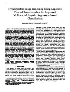
Fig. 1. True color composite for color display.
Fig. 2. CIR color composite for color display.
Fig. 3. False color composite for color display.
produce a color display that effectively conveys useful information contained in the data, most informative and distinctive bands should be selected for this purpose. Four color composite schemes using selected bands are proposed as follows. A. Scheme I: True Color Composite If three selected bands are close to the three visual primary colors, then these three bands may be combined to produce a “true color” image. In this way, the colors of the resulting color composite image resemble closely what would be observed by human eyes. In this scheme, band selection is conducted to select the most distinctive and informative band subset using a method in Section II. Then, the selected band subset is divided into three spectral regions: with the spectral segmentation (R, G, B ranges are within 610–700 nm, 500–570 nm, 450–500 nm, respectively). Finally, the three most uncorrelated bands are further selected (as described in Section III-E) and
mapped into RGB color space. The flowchart of true color composite is shown in Fig. 1. B. Scheme II: Color Infrared (CIR) Color Composite As shown in Fig. 2, Scheme II is similar to true color composite but with different spectral segmentation. In this scheme, the divided three spectral ranges are near infrared (NIR), R, and G. This scheme may be more suitable to show vegetation in an image [25]. C. Scheme III: False Color Composite In true or CIR color composite, the quality of color display may be poor since only those selected bands falling in the three specific spectral ranges can be actually used. So, if we select some informative bands without dividing the selected bands into the three spectral ranges and then map them into RGB color space, it may be a better choice. This technique is suitable if the objective is to generate a display with distinctive colors, but it
2650
IEEE JOURNAL OF SELECTED TOPICS IN APPLIED EARTH OBSERVATIONS AND REMOTE SENSING
Fig. 4. Stretched CMF composite using band selection for color display. TABLE I COMPUTATIONAL COMPLEXITY OF DIFFERENT COLOR COMPOSITE
Fig. 5. True color display using different band selection methods in Cuprite experiment. (a) MEAC; (b) LP; (c) OPD; (d) SID; (e) SAM; (f) JM.
PERFORMANCE
OF
TABLE II TRUE COLOR DISPLAY USING BAND SELECTION IN CUPRITE EXPERIMENT
— denotes the number of selected bands, and where , , and are the number of bands in three spectral regions, respectively. — denotes the number of bands, the number of classes, the number of representative pixels, the number of total training samples, and the number of total pixels.
cannot maintain consistent rendering. In order to find the most informative and uncorrelated bands, firstly, we pre-select some bands (for example 10 bands) from the original data to form a band subset ; then, select the most uncorrelated three bands from the selected bands; finally, map them into the RGB space to generate the false color image. The diagram is shown in Fig. 3. D. Scheme IV: Stretched CMF Composite In the preceding schemes, only three bands are used for color display. In fact, each band may have a specific role in hyperspectral visualization even if it includes some redundant spectral information. It was reported in [7], [25] that the three displayed R, G, and B channels, derived from linear integrations of all the original bands weighted by three different spectral envelopes, can produce consistent and robust visualization. In this section, spectral weighting envelopes based on a stretched version of the CIE 1964 tristimulus CMFs are used. For instance, in order to illuminate the Airborne Visible/Infrared Imaging Spectrometer (AVIRIS) reflectance data for display in the sRGB color space,
the CIE 1964 tristimulus color matching envelopes was transformed to the sRGB color space with its D65 white point [26], and then the wavelength scale for the envelopes was stretched to cover the AVIRIS hyperspectral range. In our case, not all the original bands are used for CMF integration. Instead, several bands are selected from the original data to form a band subset ; then these bands are multiplied by the stretched CMFs to generate the three primary colors of R, G, and B for color display. The diagram is shown in Fig. 4. E. The Strategy of Selecting a Representative Band in Each Spectral Segment When using Schemes I and II, a representative band is selected from each segment using a correlation metric, such as correlation coefficient (CC). The correlation is computed over the different spectral range of the band set . For representative band selection, the band with the highest average correlation to other bands in the same band subset is chosen as the
SU et al.: HYPERSPECTRAL IMAGE VISUALIZATION USING BAND SELECTION
2651
representative band, because it can better predict the information content of other bands. On the other hand, the selected three representative bands should have different information, compared with each other. Thus, the bands which have the highest average correlation within group and the most different information between groups are considered as the best choice for RGB color display. More specifically, an index can be computed to find the three best bands representing each region: (5) is the similarity (i.e, average CC) among the where three bands, and is the similarity of bands in the th group which can be computed as (6)
Fig. 6. CIR color display using different band selection methods in Cuprite experiment. (a) MEAC; (b) LP; (c) OPD; (d) SID; (e) SAM; (f) JM.
PERFORMANCE
OF
TABLE III CIR COLOR DISPLAY USING BAND SELECTION IN CUPRITE EXPERIMENT
where is the number of pre-selected bands in the th group. The three bands that yield the largest value of are chosen as the final bands for color display. The computational complexity of this step is approximately . F. Computational Complexity Analysis Table I lists the computational complexity of different color composites. For each method, it mainly contains two steps: band selection and color display generation. The comparison in True Color and CIR Composite are conducted among selected bands falling into different regions, while the comparison in False Color Composite is among all selected bands. So the latter has to examine more pair-wise combinations, requiring more time. It is worth mentioning that the number of selected bands required for different band selection methods in the four schemes may be different. IV. EXPERIMENTS A. Performance Evaluation For performance evaluation, the color distance between class centers (i.e. the Euclidean distance between the color vectors corresponding to class centers in the CIELab space [1]) is used for visual interpretation, and a larger average distance among class centers generally means better perceptual separation. In addition, a classifier called constrained linear discriminant analysis (CLDA) [26] is employed to generate a gray-scale classification map for each class without the requirement of training samples. When pixel-level ground truth is unavailable, each map is compared with its counterpart from using all the original bands. If they are similar, this means that the color display is satisfactory in preserving and discriminating different classes. The similarity can be assessed with average spatial correlation coefficient (CC). When training samples are available, the standard support vector machine (SVM) is applied for classification, and the classification performance is evaluated with Kappa coefficient.
Fig. 7. False color display using different band selection methods in Cuprite experiment. (a) MEAC; (b) LP; (c) OPD; (d) SID; (e) SAM; (f) JM.
PERFORMANCE
OF
TABLE IV FALSE COLOR DISPLAY USING BAND SELECTION IN CUPRITE EXPERIMENT
B. Using Other Band Selection Methods in the Proposed Models for Comparison In most of band selection algorithms, the objective is to maintain class separability when a subset of bands is selected. Class separability may be measured by: OPD [27], SID, SAM,
2652
IEEE JOURNAL OF SELECTED TOPICS IN APPLIED EARTH OBSERVATIONS AND REMOTE SENSING
Fig. 8. CMF display using different band selection methods in Cuprite experiment. (a) MEAC; (b) LP; (c) OPD; (d) SID; (e) SAM; (f) JM; (g) all bands.
TABLE V PERFORMANCE OF CMF COLOR DISPLAY IN CUPRITE EXPERIMENT
and JM. To avoid exhaustively search, the SFS search can be adopted. Note that these techniques usually require class training samples, and they measure pairwise band similarity, instead of joint similarity of multiples bands as in MEAC and LP. In this paper, OPD, SID, SAM, and JM-based band selection methods are implemented for comparison purposes. C. AVIRIS Cuprite Experiment The data used in this experiment is the AVIRIS Cuprite subimage scene sized 350 350, which was taken over Cuprite, NV, in 1997 [28]. After water absorption and low-SNR bands were removed (1–3, 105–115, and 150–170), 189 bands were left. It is known that at least five minerals were presented: alunite (A), buddingtonite (B), calcite (C), kaolinite (K), and muscovite (M). Their spectral signatures are given, which are used for MEAC band selection; for those methods requiring training samples, these signatures provide the guidance for manual training sample selection. In the true color display, the spectral segmentation is based on the traditional R, G, and B spectral ranges. So, after band selection from original data space, the bands to be mapped into the RGB space are limited to such a constraint on spectral range. Then, a representative band in each spectral range will be selected for color display according to (5). The color displays for Cuprite data using different band selection methods are shown in Fig. 5. To quantitatively evaluate the color displays, the Euclidean distance between each pair of materials in the color space was calculated and averaged, running time (in seconds) in a desktop computer with 3.10-GHz CPU and 8.0-GB memory, and the minimal numbers of selected bands to avoid an empty spectral group (BN) were also listed. As shown in Table II where the best two results are highlighted, the LP-generated color display has the largest color distance with the smallest number of bands required to search. OPD and JM have large color distances but consume more computational time because they have to search for more bands before generating the results. MEAC has the second largest color distance, and it needs to search for only 31 bands to produce the results. Also, SID band selection method has a larger color distance than OPD and JM, with less execution time. To assess object information preserved in the
color display images, the CLDA was applied to both the original data and color displays, and the average CC was computed to show the similarity between the corresponding maps as in Table II. We can see that MEAC and LP contain more material information. In CIR color composite, the spectral segmentation is based on the NIR, R, and G spectral ranges. After band selection from original data space, the selected bands are divided into these three ranges, and three bands are finally selected for color display. The color displays using different band selection methods are shown in Fig. 6. Average Euclidean distance, running time, and minimal number of selected bands to avoid an empty spectral group are shown in Table III. It can be seen that LP yields the largest color distance (23.64) with only 20 pre-selected bands, and MEAC also yields a larger color distance. From the CC values listed in Table III, we can see that LP has the highest CC value with only 2.09 seconds, while SID also has a higher value but requiring 58 pre-selected bands. Once again, LP and MEAC outperform other methods. The false color scheme aims to find the most uncorrelated three bands from the pre-selected 10 bands without any spectral segmentation. So, after 10 bands were extracted from original data, the most uncorrelated three bands will be used for color display. The color displays for Cuprite data using different band selection methods are shown in Fig. 7. Table IV tabulates the average Euclidean distance between each pair of materials in the color space, etc. It shows that LP has the highest color distance, and SID takes the second place. As listed in Table IV, LP and MEAC yield the highest CC values, which mean their color displays contain more class information. For the stretched CMF scheme, the pre-selected bands were multiplied by the spectral weighting envelopes to generate the three primary R, G, and B channels. Fig. 8 illustrates the color display results for Cuprite data using different band selection methods, where CMF on LP-selected bands and on all the original bands yield very similar display. Average Euclidean distance and CC are shown in Table V, where using LP-selected bands and using all bands have similar values of . For classification results in Table V, MEAC and LP yield competitive values of CC and running time than using all bands.
SU et al.: HYPERSPECTRAL IMAGE VISUALIZATION USING BAND SELECTION
2653
Fig. 9. True color display using different band selection methods in Indian Pines experiment. (a) MEAC; (b) LP; (c) OPD; (d) SID; (e) SAM; (f) JM.
Fig. 10. CIR color display using different band selection methods in Indian Pines experiment. (a) MEAC; (b) LP; (c) OPD; (d) SID; (e) SAM; (f) JM.
PERFORMANCE
OF
TABLE VI TRUE COLOR DISPLAY USING BAND SELECTION IN INDIAN PINES EXPERIMENT
TABLE VII PERFORMANCE
OF CIR COLOR DISPLAY USING BAND IN INDIAN PINES EXPERIMENT
SELECTION
D. AVIRIS Indian Pines Experiment The hyperspectral dataset used in this experiment is a subimage of the scene taken over the northwest Indiana’s Indian Pines test site in June 1992 [29], [30]. It has 145 145 pixels and sixteen different land-cover classes. The spatial resolution is 20 m. The data has 220 spectral bands covering 0.4–2.45 m spectral range with 10 nm spectral resolution. In the experiment, 202 out of the 220 bands are used, discarding the lower SNR bands (numbered 104–108, 150–163, and 220). Training (2074 pixels) and testing samples (8292 pixels) are available, so SVM is applied for classification. The true color displays for this data using different band selection methods are shown in Fig. 9. Table VI lists average Euclidean distance, Kappa coefficients, running time, and the minimal numbers of selected bands to avoid an empty spectral group. We can see that MEAC and LP yield the best results among all the similarity metrics. In order to produce a color display, MEAC and LP need 22 and 9 bands, respectively, but SID and SAM require 159 and 163 bands, respectively, which are more time-consuming. The Kappa values for SVM classification results are quite similar, while MEAC, LP, and SAM yield the largest value (0.49). The CIR color composites are shown in Fig. 10, and the quantitative evaluation can be found in Table VII. We can see that LP yields the higher , which means that the selected bands have better image quality for color display. In this case, the performance of JM is quite similar to those of MEAC and LP, but it is more time-consuming. The color displays using the false color scheme are shown in Fig. 11. From Table VIII, it can be seen that MEAC and LP
Fig. 11. False color display using different band selection methods in Indian Pines experiment. (a) MEAC; (b) LP; (c) OPD; (d) SID; (e) SAM; (f) JM.
PERFORMANCE
OF
TABLE VIII FALSE COLOR DISPLAY USING BAND SELECTION IN INDIAN PINES EXPERIMENT
provide the best overall performance with much less execution time. For the stretched CMF scheme, the color displays are shown in Fig. 12. The displays from MEAC, LP, SID, and all bands look more similar with the same tones. As listed in Table IX,
2654
IEEE JOURNAL OF SELECTED TOPICS IN APPLIED EARTH OBSERVATIONS AND REMOTE SENSING
Fig. 12. CMF display using different band selection methods in Indian Pines experiment. (a) MEAC; (b) LP; (c) OPD; (d) SID; (e) SAM; (f) JM; (g) all bands.
TABLE IX PERFORMANCE OF CMF COLOR DISPLAY IN INDIAN PINES EXPERIMENT
TABLE X COMPARISON OF DIFFERENT COLOR COMPOSITE MODELS USING SELECTED BANDS
for average Euclidean distance, MEAC and LP take the first two places with the largest values; except , using MEAC or LP-selected bands produce the similar results as using all bands. E. Comparison Among the Proposed Models Additional two hyperspectral data [30] were used for performance evaluation. One dataset is collected by the ROSIS optical sensor over the urban area of the University of Pavia, Italy, the image size in pixels is 610 340, with a very high spatial resolution of 1.3 m per pixel. The number of data channels in the acquired image is 103 (with spectral range from 0.43 to 0.86 m). It contains 9 classes. The other dataset was collected by the 224-band AVIRIS sensor over Salinas Valley, California, and is characterized by high spatial resolution (3.7-meter pixels). The area covered comprises 512 lines by 217 samples. As with the Indian Pines scene, we discarded the 20 water absorption bands. This image was available only as at-sensor radiance data. It includes 16 classes such as vegetables, bare soils, vineyard fields, etc.
In order to compare the performance of the four proposed color composite schemes, Table X summarizes the experimental results of , CC (or Kappa coefficients), BN, and computing time. The two best scores in each case are highlighted. As mentioned earlier, except the false color model, all the other three models have the property of consistent rendering. Using false color model, color distance is generally larger. As for class separability, the false color model did better in the Cuprite experiment; while the CMF model produced larger Kappa coefficients in other experiments. Note that the CMF model here uses selected bands, not all bands; as shown earlier, using selected bands can provide better results. As for MEAC and LP, the performance of LP is slightly better. F. Comparison With Other Color Display Methods To further evaluate the performance of the proposed algorithms, some color display methods in the literature, such as PCA [4] and 1BT [6], are implemented. In the 1BT method, three bands are determined and retained for RGB display using one-bit transform band selection method. For PCA-based visualization,
SU et al.: HYPERSPECTRAL IMAGE VISUALIZATION USING BAND SELECTION
2655
the first three principal components are mapped to the RGB color space. The visualization results for the proposed LP approach, 1BT, and PCA based approach for the four datasets are shown in Fig. 13, where only LP (false color) and LP (CMF) are presented since they provided overall the best performance in Section IV-E. It can be seen that the color display images of PCA and 1BT for Indian Pines data look a little obscure. As listed in Table XI, LP (false color) generally provides large values, while LP (CMF) yields better classification performance.
[12] H. Yang, Q. Du, H. Su, and Y. Sheng, “An efficient method for supervised hyperspectral band selection,” IEEE Geosci. Remote Sens. Lett., vol. 8, no. 1, pp. 138–142, 2011. [13] Q. Du and H. Yang, “Similarity-based unsupervised band selection for hyperspectral image analysis,” IEEE Geosci. Remote Sens. Lett., vol. 5, no. 4, pp. 564–568, 2008. [14] H. Yang, Q. Du, and G. Chen, “Unsupervised hyperspectral band selection using graphics processing units,” IEEE J. Sel. Topics Earth Observ. Remote Sens., vol. 4, no. 3, pp. 660–668, 2011. [15] R. Pouncey, K. Swanson, and K. Hart, ERDAS Field Guide, 5th ed. Atlanta, GA, USA: ERDAS Inc., 1999. [16] J. A. Richards and X. Jia, Remote Sensing Digital Image Analysis: An Introduction, 4th ed. Berlin, Germany: Springer-Verlag, 2006, ch. 10, pp. 267–292. [17] A. Ifarraguerri, “Visual method for spectral band selection,” IEEE Geosci. Remote Sens. Lett., vol. 1, no. 2, pp. 101–106, 2004. [18] C.-I Chang, Hyperspectral Imaging: Techniques for Spectral Detection and Classification. New York, NY, USA: Kluwer, 2003, ch. 2, pp. 15–35. [19] P. Bajcsy and P. Groves, “Methodology for hyperspectral band selection,” Photogramm. Eng. Remote Sens., vol. 70, no. 7, pp. 793–802, 2004. [20] C.-I Chang, Q. Du, T.-L. Sun, and M. L. G. Althouse, “A joint band prioritization and band decorrelation approach to band selection for hyperspectral image classification,” IEEE Trans. Geosci. Remote Sens., vol. 37, no. 6, pp. 2631–2641, 1999. [21] N. Keshava, “Distance metrics and band selection in hyperspectral Processing with applications to material identification and spectral libraries,” IEEE Trans. Geosci. Remote Sens., vol. 42, no. 7, pp. 1552–1565, 2004. [22] C. Conese and F. Maselli, “Selection of optimum bands from TM scenes through mutual information analysis,” ISPRS J. Photogramm. Remote Sens., vol. 48, no. 3, pp. 2–11, 1993. [23] S. S. Shen and E. M. Bassett, “Information theory based band selection and utility evaluation for reflective spectray systems,” in Proc. SPIE, 2002, vol. 4725, pp. 18–29. [24] P. Pudil, F. J. Ferri, J. Novovicova, and J. Kittler, “Floating search methods for feature selection with nonmonotonic criterion functions,” in Proc. 12th Int. Conf. Pattern Recognition, IAPR, 1994, pp. 279–283. [25] S. C. Liew, Space View of Asia, 2nd ed. Singapore: National University of Singapore, 1997. [26] Q. Du and C.-I Chang, “Linear constrained distance-based discriminant analysis for hyperspectral image classification,” Pattern Recognition, vol. 34, no. 2, pp. 361–373, 2001. [27] H. Su, Y. Sheng, H. Yang, and Q. Du, “Orthogonal projection divergence-based hyperspectral band selection,” Spectroscopy and Spectral Analysis, vol. 31, no. 5, pp. 1309–1313, 2011. [28] Aviris. Jet Propulsion Lab, California Inst. Technol. [Online]. Available: http://aviris.jpl.nasa.gov/data/free_data.html [29] MultiSpec. Purdue Research Foundation, 1994 [Online]. Available: https://engineering.purdue.edu/~biehl/MultiSpec/hyperspectral.html [30] Hyperspectral Remote Sensing Scenes. [Online]. Available: http://www.ehu.es/ccwintco/index.php/Hyperspectral_Remote_ Sensing_Scenes
V. CONCLUSION In this paper, we investigate four color composite schemes for hyperspectral image visualization using pre-selected bands. From the real data experiments, we can conclude that MEAC and LP-based color display methods provide overall robust performance in terms of image quality and class separability. In addition, they can provide very fast and better color display results with the support of the proposed four color composite schemes. Among the four schemes, the CMF model using selected bands produces the overall best performance (i.e., higher classification accuracy in the RGB space, larger color distance in the CIELab space, while maintaining consistent rendering), which is also better than the original CMF model using all the original bands. It is shown that such band selection-based color composite schemes are the simple but efficient technique for hyperspectral image visualization. REFERENCES [1] Q. Du, N. Raksuntorn, S. Cai, and R. J. Moorhead, “Color display for hyperspectral imagery,” IEEE Trans. Geosci. Remote Sens., vol. 46, no. 6, pp. 1858–1866, 2008. [2] G. Poldera and G. W. A. M. van der Heijden, “Visualization of spectral images,” in Proc. SPIE, 2001, vol. 4553, p. 133. [3] N. P. Jacobson and M. R. Gupta, “Design goals and solutions for display of hyperspectral images,” IEEE Trans. Geosci. Remote Sens., vol. 43, no. 11, pp. 2684–2692, 2005. [4] J. S. Tyo, A. Konsolakis, D. I. Diersen, and R. C. Olsen, “Principal components-based display strategy for spectral imagery,” IEEE Trans. Geosci. Remote Sens., vol. 41, no. 3, pp. 708–718, 2003. [5] N. P. Jacobson, M. R. Gupta, and J. B. Code, “Linear fusion of image sets for display,” IEEE Trans. Geosci. Remote Sens., vol. 45, no. 10, pp. 3277–3288, 2007. [6] B. Demir, A. Celebi, and S. Erturk, “A low-complexity approach for the color display of hyperspectral remote-sensing images using one-bittransform-based band selection,” IEEE Trans. Geosci. Remote Sens., vol. 47, no. 1, pt. 1, pp. 97–105, 2009. [7] S. Le Moan, A. Mansouri, Y. Voisin, and J. Y. Hardeberg, “A constrained band selection method based on information measures for spectral image color visualization,” IEEE Trans. Geosci. Remote Sens., vol. 49, no. 12, pp. 5104–5115, 2011. [8] S. Le Moan, A. Mansouri, J. Y. Hardeberg, and Y. Voisin, “Visualization of spectral images: A comparative study,” in PCSPA/GCIS, Gjovik, Norway, 2011. [9] B. Guo, S. R. Gunn, R. I. Damper, and J. B. Nelson, “Band selection for hyperspectral image classification using mutual information,” IEEE Geosci. Remote Sens. Lett., vol. 3, no. 4, pp. 522–526, 2006. [10] C.-I Chang, “An information-theoretic approach to spectral variability, similarity, discrimination for hyperspectral image analysis,” IEEE Trans. Inf. Theory, vol. 46, no. 5, pp. 1927–1932, 2000. [11] H. Su, H. Yang, Q. Du, and Y. Sheng, “Semi-supervised band clustering for dimensionality reduction of hyperspectral imagery,” IEEE Geosci. Remote Sens. Lett., vol. 8, no. 6, pp. 1135–1139, 2011.
Hongjun Su (S’09–M’11) received the B.S. degree in geography information system from the China University of Mining and Technology in 2006, and the Ph.D. in cartography and geography information system from the Key Laboratory of Virtual Geographic Environment (Ministry of Education), Nanjing Normal University, China, in 2011. He was a visiting student in the Department of Electrical and Computer Engineering at Mississippi State University, Starkville, MS, USA, from 2009 to 2010. He is now working at the School of Earth Sciences and Engineering, Hohai University, Nanjing, China. He also with the Department of Geographical Information Science, Nanjing University, as a postdoctoral fellow. His main research interests include hyperspectral remote sensing dimensionality reduction, classification, and spectral unmxing. Dr. Su is an active reviewer for the IEEE TRANSACTIONS ON GEOSCIENCE AND REMOTE SENSING, the IEEE Geoscience and Remote Sensing Letters, the IEEE JOURNAL OF SELECTED TOPICS IN APPLIED EARTH OBSERVATIONS AND REMOTE SENSING, the International Journal of Remote Sensing, and the Optics Express.
2656
IEEE JOURNAL OF SELECTED TOPICS IN APPLIED EARTH OBSERVATIONS AND REMOTE SENSING
Qian (Jenny) Du (S’98–M’00–SM’05) received the Ph.D. degree in electrical engineering from the University of Maryland Baltimore County, USA, in 2000. She is the Bobby Shackouls Professor in the Department of Electrical and Computer Engineering at Mississippi State University, Starkville, MS, USA. Her research interests include hyperspectral remote sensing image analysis, pattern classification, data compression, and neural networks. Dr. Du serves as Co-Chair for the Data Fusion Technical Committee of IEEE Geoscience and Remote Sensing Society (GRSS) (2009–2013), and Chair for Remote Sensing and Mapping Technical Committee of International Association for Pattern Recognition (IAPR). She also serves as an Associate Editor for IEEE JOURNAL OF SELECTED TOPICS IN APPLIED EARTH OBSERVATIONS AND REMOTE SENSING and an Associate Editor for IEEE Signal Processing Letters. She is the guest editor for several journal special issues on remote sensing data processing and analysis. She received the 2010 Best Reviewer Award from IEEE GRSS for her service to IEEE Geoscience and Remote Sensing Letters. She is the General Chair of the 4th GRSS Workshop on Hyperspectral Image and Signal Processing: Evolution in Remote Sensing (WHISPERS).
Peijun Du (M’07–SM’12) is a Professor of Photogrammetry and Remote Sensing at the Department of Geographic information Sciences, Nanjing University, China, and the Deputy Director of the Key Laboratory for Satellite Surveying Technology and Applications of National Administration of Surveying and Geoinformation, China. He also serves as the Associate Editor of IEEE Geoscience and Remote Sensing Letters (GRSL). After receiving his Ph.D. degree from China University of Mining and Technology in 2001, he was employed as a teacher by this university until he joined Nanjing University in 2011. He was a postdoctoral fellow at Shanghai Jiao Tong University from February 2002 to March 2004, and was a visiting scholar at the University of Nottingham during November 2006 to November 2007. His research interests are remote sensing image processing and pattern recognition; remote sensing applications; hyperspectral remote sensing information processing; multi-source geospatial information fusion and spatial data handling; integration and applications of geospatial information technologies; and environmental information science (environmental informatics). He has published nine textbooks in Chinese and more than 120 research articles about remote sensing and geospatial information processing and applications. Dr. Du is the Co-chair of the Technical Committee, URBAN 2009 (the 5th IEEE GRSS/ISPRS Joint Workshop on Remote Sensing and Data Fusion over Urban Areas) and IAPR PRRS 2012, and the Co-chair of the Local Organizing Committee of JURSE 2009, WHISPERS 2012 and EORSA 2012. He also serves as a member of the scientific committee or technical committee of other international conferences, for example, Spatial Accuracy 2008, ACRS 2009, WHISPERS 2010, 2011, 2012 and 2013, URBAN 2011 and 2013, MultiTemp 2011 and 2013, and ISDIF 2011, SPIE Remote Sensing (Conference 07) 2012 and 2013. He is also a senior member of IEEE GRSS, a council member of China Society for Image and Graphics (CSIG), and a council member of China Association for Remote Sensing Applications (CARSA).
SU et al.: HYPERSPECTRAL IMAGE VISUALIZATION USING BAND SELECTION
Fig. 13. Color display using different methods. (a) Cuprite; (b) Indian Pines; (c) University of Pavia; (d) Salinas.
2657
2658
IEEE JOURNAL OF SELECTED TOPICS IN APPLIED EARTH OBSERVATIONS AND REMOTE SENSING
TABLE XI COMPARISON OF DIFFERENT COLOR DISPLAY APPROACHES