Unsupervised Hyperspectral Band Selection Using ... - CiteSeerX
Recommend Documents
Also, dual-tree complex wavelet transform was used to remove the spectral noise ..... AVIRIS sensor over the Kennedy Space Center (KSC), Florida, on March 23, 1996 [50]. ..... demic Visitor with the Department of Electrical En- gineering and ...
âreal-life imageâ) usually carries considerable degree of regu- larity. Meanwhile, the spectrum of woods is also chosen for the illustration of the automatic spatial ...
By. ALINA ZARE. A DISSERTATION PRESENTED TO THE GRADUATE SCHOOL. OF THE UNIVERSITY OF FLORIDA IN PARTIAL FULFILLMENT .... TECHNICAL APPROACH . ...... The min and max auto-associative memories are related.
Accepted to IEEE Geoscience and Remote Sensing Letters - GRSL-00189-2007.R2. 1. Abstractâ This paper presents a simultaneous band selection.
Hongjun Su, Member, IEEE, Qian Du, Senior Member, IEEE, and Peijun Du, Senior ... at http://ieeexplore.ieee.org. ...... and Remote Sensing Letters (GRSL).
where M and D are the number of bands before and after band selection, respectively. This dimensionality reduction problem can be modeled as a special ...
AbstractâAn improved firefly algorithm (FA)-based band se- lection method is proposed for hyperspectral dimensionality re- duction (DR). In this letter, DR is ...
approaches. However, considering the immense number of possible band combinations, the computational cost is still prohibitively high and such approaches ...
number of features and a validity index that measures the quality of clusters ..... S3. 3. 0.051891. 3. 1, 3, and 4. S4. 3. 0.073910. 2. 1 and 4. S5. 3. 0.206899. 1. 3.
May 4, 2012 - The objective of hyperspectral band selection is to select a subset of ... of PSO in band selection area,9,10 where the number of particles.
As a result, the proposed CBS using the concept of the CEM to linearly constrain a band image, while also minimizing band correlation or dependence provided.
Sep 28, 2012 - [15] Hui Wang, David Bell, and Fionn Murtagh, âFeature subset selection based on relevanceâ , Vistas in Astronomy, Volume 41, Issue 3, 1997,.
To test the concept of band selection from hyperspectral data for a multispectral .... If the desired number of bands is not obtained, go to step 1, otherwise band ...
Aug 1, 2014 - Image Based on Data Quality. Kang Sun, Xiurui Geng, Luyan Ji, and Yun Lu. AbstractâMost unsupervised band selection methods take the.
context of hyperspectral data analysis, determination of informative bands .... A cluster analysis in the ..... Varshney,P.K., Arora,M.K. âAdvanced Image Processing.
However, in the previous work using. ICA,3) the authors supposed that the number of materials in an n-band hyperspectral-image is m and considered m pure.
Representative Band Selection for Hyperspectral ... - MDPI › publication › fulltext › 32716245... › publication › fulltext › 32716245...by F Xie · 2018 · Cited by 11 · Related articlesAug 22, 2018 — hybrid filter-wrapper band selection method is p
optimal feature size by employing the HySime algorithm in the PS. ... See http://www.ieee.org/publications_standards/publications/rights/index.html for more ...
We use a one-hour forum for TV program that is broadcast on Sun- days as the ..... [4] S. Chen and P. Gopalakrishnan, âSpeaker, Environment and. Channel ...
Abstract. Background: Classification of biological samples of gene expression data is a basic building block in solving several problems in the field of ...
trix A, ai means the i-th row vector of A, Aij denotes the. (i, j)-th entry of A, â¥Aâ¥F is ..... 4http://www.cs.nyu.e
Hierarchical Classifier and Tabu Search. Donna Korycinski1, Melba Crawford1, J.W. Barnes2, Joydeep Ghosh3. 1Center for Space Research, University of ...
S.-S. Chiang and C.-I Chang are with the Remote Sensing Signal and Image ... by centering the original data matrix using a linear translation followed by an ...
The aim of this paper is to apply unsupervised feature selection to text data. ..... TER, BASE and SUPERVISED are compared on test set accuracy from a retrieve-only ... hard drive) can be used in reference to both classes (i.e. PC and Apple.
Unsupervised Hyperspectral Band Selection Using ... - CiteSeerX
G. Chen is with DCM Research Resources LLC, Germantown, MD 20874. USA. Color versions of one or more of the figures in this paper are available online.
660
IEEE JOURNAL OF SELECTED TOPICS IN APPLIED EARTH OBSERVATIONS AND REMOTE SENSING, VOL. 4, NO. 3, SEPTEMBER 2011
Unsupervised Hyperspectral Band Selection Using Graphics Processing Units He Yang, Student Member, IEEE, Qian Du, Senior Member, IEEE, and Genshe Chen, Member, IEEE
Abstract—The high dimensionality of hyperspectral imagery challenges image processing and analysis. Band selection is a common technique for dimensionality reduction. When the desired object information is unknown, an unsupervised band selection approach is employed to select the most distinctive and informative bands. Although band selection can significantly alleviate the computational burden in the following data processing and analysis, the process itself may induce additional computation complexity, especially when the image spatial size is large; it may be time-consuming for unsupervised band selection methods that need to take all pixels into consideration. Parallel computing techniques are widely adopted to alleviate the computational burden and to achieve real-time processing of data with vast volume. In this paper, we propose parallel implementations via emerging general-purpose graphics processing units (GPUs) for band selection without changing band selection result. Its speedup performance is comparable to the cluster-based parallel implementation. We also propose an approach to using several selected pixels for unsupervised band selection and the number of pixels needed can be equal to the number of selected bands minus one. With whitened pixel signatures (not the original pixels), band selection performance can be comparable to or even better than that from using all the pixels. For this approach, parallel computing is implemented for pixel selection only, since computational complexity in band selection has been greatly reduced. Index Terms—Band selection, graphics computing units (GPUs), high performance computing, hyperspectral imagery, parallel computing.
I. INTRODUCTION
B
AND selection is a frequently used dimensionality reduction technique for hyperspectral imagery. It selects a subset of original bands without losing their physical meaning. Supervised and unsupervised band selection techniques have been widely studied [1]–[8]. Compared to supervised band selection techniques, unsupervised methods need no priori information about objects or classes [9], [10]. In general, they are more practical than supervised methods. However, unsupervised methods may need to analyze the whole dataset, resulting in higher computation complexity than supervised ones that Manuscript received September 01, 2010; revised January 11, 2011; accepted February 19, 2011. Date of publication April 07, 2011; date of current version August 26, 2011. H. Yang and Q. Du are with the Geosystems Research Institute of High Performance Computing Collaboratory and the Department of Electrical and Computer Engineering, Mississippi State University, Mississippi State, MS 39762 USA (e-mail: [email protected]). G. Chen is with DCM Research Resources LLC, Germantown, MD 20874 USA. Color versions of one or more of the figures in this paper are available online at http://ieeexplore.ieee.org. Digital Object Identifier 10.1109/JSTARS.2011.2120598
may need to consider a limited number of object signatures or class samples only. In this research, we focus on unsupervised band selection. A series of unsupervised band selection methods were compared in [5]. For instance, first-spectral derivative (FSD) and uniform spectral spacing (USS) can be easily implemented with superior performance in general. Principal component analysis (PCA) [1], noise-adjusted PCA (NAPCA) [1], independent component analysis (ICA) [18], and discrete wavelet transform [19] were proposed for unsupervised band selection; distance-based measurement was investigated in [6]; and information theory-based band selection can be found in [7], [8]. Since the basic idea of unsupervised band selection methods is to find the most distinctive and informative bands, the approaches that are proposed to search for distinctive spectral signatures as endmembers can be applied. The major difference is that the algorithms are applied in the spatial domain for band selection instead of in the spectral domain for endmember extraction. There are quite a few endmember extraction algorithms existing. In general, endmember extraction algorithms can be divided into two categories: one extracting distinctive pixels based on similarity measurement, and the one using the geometry concept, such as simplex. The endmember extraction algorithm using unsupervised fully constrained linear unmxing (FCLSLU) in [11] belongs to the first category, while the well-known N-FINDR algorithm [12] belongs to the second category. In [9], the concept of N-FINDR was applied to band selection and obtained promising results. In [10], we have proposed a band selection algorithm using band linear prediction (LP), which used the similar idea of unconstrained least squares linear unmixing (UCLSLU) in endmember selection. We have demonstrated that the LP-based method in conjunction with data whitening can outperform other widely used band selection approaches [10]. Thus, we will focus on this method hereafter. To alleviate the computational burden of unsupervised band selection, it is desirable to implement such algorithms in parallel when parallel computing facilities are available. Clusters are widely used for high performance computing. However, clusters are usually expensive and cannot be employed for onboard processing due to its weight, heat dissipation, and energy consumption issues. Recently, graphics computing units (GPUs) are of great interest to high performance computing community because it can provide very high levels of computing performance at very low cost; in particular, it is suitable to real-time onboard processing due to its portability. Although it is originally specified for computer graphics, it is now popular for general-purpose computing [13]. GPU has been applied to hyperspectral image analysis, such as detection, classification, and unmixing [14]–[16], [22]. In this paper, we propose GPU implementations
YANG et al.: UNSUPERVISED HYPERSPECTRAL BAND SELECTION USING GRAPHICS PROCESSING UNITS
for unsupervised band selection. We evaluate the performance of the GPU implementations and compare it with the cluster implementation. II. SIMILARITY-BASED UNSUPERVISED BAND SELECTION In this section, we briefly introduce the LP-based and N-FINDR-based band selection methods. The objective is to find the most dissimilar bands, adopting the same idea of extracting the most dissimilar pixels as endmembers. Pixel selection using N-FINDR-based endmember extraction is also discussed. For clarification purpose, N-FINDR-based band , and N-FINDR-based endselection is denoted as member extraction for pixel selection is denoted as . When the superscript “e” or “b” is absent, it means the related description is suitable to either case. A. LP-Based Band Selection To select the most distinctive but informative bands, water absorption and low signal-to-noise ratio (SNR) bands need to be pre-removed. This is because they can be very distinctive but not informative. The noise component in different bands is varied. If the noise component is larger, a band may look more different from others although it may not be informatively distinct. So noise whitening is needed which requires noise estimation. It is known that noise estimation is a difficult task. Therefore, we apply data whitening to the original bands (after bad band removal) as an alternative, which can be easily achieved by the eigen-decomposition of data covariance matrix . Then the whitened bands actually participate in the following band selection process. Note that the selected bands are the original not the whitened ones. To select the distinctive bands or the most dissimilar bands, a similarity metric needs to be designated. The widely used metrics include distance, correlation, etc. The measurement is taken on each pair of bands. Here, we prefer to use the approaches where band similarity is evaluated jointly instead of pair-wisely. The proposed band selection algorithms using the same concept in endmember extraction has this property. In addition, due to the large number of original bands, the exhaustive search for optimal band combinations is computationally prohibitive. The sequential forward search can save significant computation time. It begins with the best two-band combination, and then this two-band combination is subsequently augmented to three, four, and so on, until the desired number of bands is selected. The studied band selection algorithms using the endmember extraction concept adopt this sequential forward search strategy. Another advantage is that it is less dependent on the number of bands to be selected, since those bands already being selected do not change with this value; increasing this value simply means to continue the algorithm execution with the bands being selected while decreasing this number simply means to keep enough bands from the selected band subset (starting with the first selected band) as the final result. The basic steps can be described as below. 1) Initialize the algorithm by choosing a pair of bands and . Then the resulting selected band subset is .
661
that is the most dissimilar to all the 2) Find a third band bands in the current using a certain criterion. Then the . selected band subset is updated as 3) Continue on step 2) until the number of bands in is large enough. The straightforward criterion that can be employed for similarity comparison is LP, which can jointly evaluate the similarity between a single band and multiple bands. The concept in the LP-based band selection was originally used in the FCLSLU for endmember pixel selection in [11], which means a pixel with the maximum reconstruction error using the linear combination of existing endmember pixels is the most distinctive pixel. The difference here is that for band selection there is no constraint imposed on the coefficients of linear combination. and in with pixels Assume there are two bands each. To find a band that is the most dissimilar to and , and are used to estimate a third band , i.e., (1) where is the estimate or linear prediction of band using and , and , , and are the parameters that can minimize . Let the parameter the linear prediction error: vector be . The matrix form of (1) is (2) and
can be determined using a least-squares solution: (3)
where is an matrix whose first column is 1, second pixels in , third column includes column includes all the vector with all the pixels all the pixels in , and is an in . The band that yields the maximum error (using the optimal parameters in ) is considered as the most dissimilar and and will be selected as for . Obviously, band to the similar procedure can be easily conducted when the number of bands in is larger than two. The number of bands to be selected can be pre-estimated by the virtual dimensionality estimation methods in [23]. However, this is not critical in the LP algorithm because of the sequential forward searching strategy being deployed. In other words, if bands are selected, the -th band can be selected based on the first bands; or if bands have been selected, to select bands , just take the first bands of . The original LP-based band selection algorithm uses all the pixels. To reduce computational complexity, it can use several (denoted as ) selected pixels with as described in Section II-B. B. N-FINDR-Based Pixel Selection via Endmember Extraction The major problem of the LP-based band selection is that computational cost is high if all the pixels are used. The N-FINDR algorithm can be applied for pixel selection, and then the selected pixels are used for band selection. The basic idea of the original N-FINDR algorithm is to find the pixels that can construct a simplex with the maximum volume and these pixels will be considered as endmembers. Due to the mathematical
662
IEEE JOURNAL OF SELECTED TOPICS IN APPLIED EARTH OBSERVATIONS AND REMOTE SENSING, VOL. 4, NO. 3, SEPTEMBER 2011
intractability, only an estimate of the optimal solution can be found. A greedy-type algorithm can be described as follows. be the number of endmembers to be gener1) Let ated. The original -dimensional hyperspectral image is reduced to -dimensional using PCA or Maximum Noise Fraction (MNF) transform. be a set of initial 2) Let vectors randomly or carefully selected from the data, constructing a simplex [17]. The volume of the simplex can be calculated as (4) where
and
de-
notes matrix determinant operation. 3) At the -th stage, use the -th pixel to replace each individual endmember as a new simplex vertex and compute the resulting volume. If the maximum volume is larger than in the previous step and it appears when is replaced by , then is used as ; otherwise, go to -th stage to test the -th pixel . the 4) The algorithm is stopped when all the pixels are tested. C. N-FINDR-Based Band Selection As mentioned in Section II-A, an endmember extraction algorithm can be applied for band selection. So the N-FINDR algorithm can be run in the spatial domain for band selection in [9]. It was demonstrated that using data whitening can improve band -based selection performance in [10]. However, the band selection is difficult to be implemented with all the pixels matrix has to be evaluated, where is the since an number of pixels. Thus, a small precentage of pixels can be randomly chosen for band selection as in [9], [10]. Another strategy is to find distinctive pixels for band selection as presented in Section II-B. Note that when only several pixels are selected for band selection, data whitening is not applied by any more due to the ill-ranked data covariance matrix. -based band selection algorithm in [10] can The be described as follows. pixels for band selection. Con1) Randomly select duct data whitening. All bands (with selected pixels) are stacking into column vectors. 2) Assume bands to be selected. Randomly select bands as the initials. Or use the iterative error analysis (IEA) algorithm to pick up the most distinctive band vectors [25]. principal compo3) Conduct PCA and choose the first nents. 4) Run the N-FINDR algorithm in Section II-B (steps 2–4) to finalize the band vectors. -based band seIn this paper, we propose the selected pixels (denoted lection algorithm using ) that can be described as below, as where no data whitening or PCA are needed during band selection. pixels for 1) Assume bands to be selected. Select -based pixel selection. All band selection using
bands (with selected pixels only) are stacked into column vectors. 2) Randomly select bands as the initials. Or use the IEA algorithm to pick up the most distinctive band vectors. 3) Run the N-FINDR algorithm in Section II-B (steps 2–4) to finalize the band vectors. D. About Data Whitening Process for Band Selection As discussed in [10], a data whitening process can improve unsupervised band selection performance because it can help extract truly informative bands. When using several selected for band selection, data whitening pixels from the is not applicable any more as mentioned in Section II-C. However, we can use the pixel signatures in the whitened data for band selection instead of the pixels in the original data. In the experiment, we will show that the use of whitened pixel signatures can improve the performance. It is noteworthy that our algorithm is applied on the whitened data because the standard PCA (data decorrelation followed by variance normalization) is adopted in the dimensionality reduction process, or LP for band selecso using whitened pixels in tion does not incur extra computing cost. E. Strategies for Saving Computational Cost Before implementing the aforementioned algorithms in parallel, several strategies (in addition to pixel selection) to saving computational cost are discussed as below. They can greatly save time for the original series versions; in addition, they can significantly improve the speedup performance for the parallel versions. Saving Computational Cost for LP Method: The key step in the LP method is to solve the coefficients as in (3). Let denote , the data matrix constructed by the selected bands of size unselected bands. Similar and denote the one about sets of coefficients of size are to (3), the calculated as (5) and the of the matrix
prediction residuals are the column-wise norms
(6) Since , the computation cost of solving the LP coeffiof cients is dominated by forming the symmetric matrix and the matrix of size . Notice that size and are both subsets of the entire data correlation matrix of size . They can be retrieved from without any calculation in each step. In each iteration only one band is added to and deleted from , and only one row needs to be updated for and . includes multiplicaThe calculation of the entire tions, and many items in may not be used in an actual band selection process. However, the noise whitening step needs to compute the covariance matrix and it is related to as (7)
YANG et al.: UNSUPERVISED HYPERSPECTRAL BAND SELECTION USING GRAPHICS PROCESSING UNITS
663
where is the data mean vector. Thus, additional cost in calculation is negligible. Saving Computational Cost for N-FINDR Method: The major computational cost in the N-FINDR is for matrix determinant calculation in (4). In a specific run, an endmember is replaced by pixels one after another with other endmembers being fixed. Thus, matrix determinant calculation can take advantage of unchanged determinants of submatrices, i.e., is replaced by all the pixels, the rest of cofactors. When the matrix remains the same. With cofactor expansion, the determinant can be computed as
.. .
.. .
..
.
.. .
(8) is the -th minor, the determinant of the submawhere constructed by removing the -th row and -th column trix of , which can be reused when updating . Note that some recent work on N-FINDR parallel implementation can be found in [20], [21]. Our implementation with cofactor-expansion-related computation can result in tremendous savings in both serial and parallel versions. Fig. 1. Parallel LP band selection algorithm.
III. GPU IMPLEMENTATIONS The GPU is usually treated as a parallel computer with shared memory architecture. As all processors of the GPU can share data within a global address space, it fits the data parallelism very well. To achieve satisfied parallel performance, the data throughput is very critical in GPU parallel algorithm design, which means enough data should be fed into the GPU to take advantage of computing power. Many previous work shows that it can achieve excellent speedup performance only when the data size is increased to thousands. As it uses the share memory model, the major bottleneck is memory communication between the host and device; unnecessary data transfer between host and device should be avoided. In other words, the most data computation should take place in GPU without interruption. While data sharing between GPU cores is much easier than clusters, the data throughput requirement makes current GPUs inappropriate for solving a bunch of small matrix operation problems. Therefore, two key rules of GPU parallelization are followed: 1) to parallelize a large number of scalar/vector additions/multiplications if possible, and 2) to reduce communications between host and device as much as possible. In hyperspectral image processing, the spatial size of an image is much larger than the spectral size, which suggests to fulfilling computation tasks in spatial order on GPU while leaving other tasks (such as small matrix manipulations) to CPU. In this way, the workload between the GPU and the CPU can be well balanced. Our algorithms use matrix operations extensively. Fortunately, the CUDA CUBLAS library provides high performance
computing implementation for the Basic Linear Algebra Subprograms (BLAS) level 1 to level 3 operations [24]. Thus, our parallel algorithms are designed to utilize the existing parallel linear algebra library, which requires to keeping data continuity in the memory as much as possible. Thus, we mainly discuss how to avoid breaking data continuity and to save unnecessary data movement hereafter. The flow chart for the GPU implementation of the LP-based band selection algorithm is shown in Fig. 1. It is similar to the serial version although it needs to send data back and forth between the host (CPU) and the device (GPU). Since the spatial size of hyperspectral data is much larger than its spectral size, data computational tasks directly related to pixel vectors (e.g., correlation and covariance matrix calculation) is given to the GPU and those related to matrix manipulations (e.g., matrix inversion) are given to the CPU; the former has the order equal to the number of pixels and the latter has the order equal to the number of bands. To further reduce computational burden, proper data structure is designed to avoid unnecessary data communication and maintain data locality. As illustrated in Fig. 2, data is saved in column-major order, and each band is stacking into a column; after one band is selected in each iteration, the selected band is swapped with the last member of the unselected set of bands. To avoid calculating band correlation items in and repeatedly, the corresponding rows and columns in are also swapped and rethe entire data correlation matrix and update. This concept is illustrated in trieved for
664
IEEE JOURNAL OF SELECTED TOPICS IN APPLIED EARTH OBSERVATIONS AND REMOTE SENSING, VOL. 4, NO. 3, SEPTEMBER 2011
Fig. 2. Illustration of data manipulation for parallel implementation. (with the case that the total number of bands is four).
Fig. 4. Parallel
N-FINDR
algorithm.
the volumes resulting from replacing an endmember with dif-based ferent pixels are examined by GPU. Parallel band selection has the similar structure as the parallel LP band -based band selection uses a selection. Actually, few selected pixels only; thus, serial band selection may be even faster than the parallel version. IV. EXPERIMENTS Fig. 3. Illustration of matrix manipulation in Eq. (6) for LP parallel implementation. Assumed there are four bands. At the beginning: f ; ; ; g, ; after the first step: f ; ; g, f g; after the second step: f ; g, f ; g.
B B B B S= B
S =
U = U = B B B
U= B B S= B B
Fig. 3 with the total number band being four. Data swapping ensures data continuity for both selected bands in and unselected bands in , which makes the following prediction residual evaluation with in (6) more efficiently. The flow chart for the GPU implementation of the -based pixel selection is shown in Fig. 4. To fully take advantage of GPU computing power and reduce unnecessary host/device communication overhead, the large size of matrix/vector multiplications, such as principal component transform, are conducted in GPU, while the manipulations of relatively small matrices, such as eigen-decomposition of data covariance matrix , is left for CPU. Similarly, when calculating simplex volumes, cofactors are computed by CPU;
A. Computing Facilities and Dataset The CPU machine used in the experiments is an Intel Pentium4 3.40 GHz with Hyper thread and 2 GB of memory. The GPU is NVidia’s GeForce GTX285 that has 240 cores with 1 GB memory. The Linux-based cluster used in the experiments has 384 processors, which is composed by 192 IBM xSeries x335 servers and each with two 3.06 GHz Xeon processors and 2.5 GB of memory; each of the nodes is diskless and connected to the cluster’s internal network via InfiniBand with very high speed (10 gigabits per second) and very low latency network architecture. The parallel algorithms on the cluster are implemented in the C++ with the message passing interface (MPI) and Intel’s Math Kernel Library (MKL) version 10.1. The GPU versions are implemented in the C++ with CUBLAS and MKL version 11.1. All algorithms use double precision.
YANG et al.: UNSUPERVISED HYPERSPECTRAL BAND SELECTION USING GRAPHICS PROCESSING UNITS
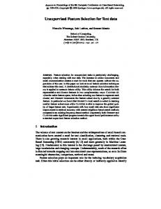
Fig. 5. An AVIRIS Cuprite scene including minerals named as: alunite (A), buddingtonite (B), calcite (C), kaolinite (K), and muscovite (M).
665
Fig. 6. Speedup of the parallel LP band selection algorithm.
TABLE I PARALLEL LP-BASED BAND SELECTION RUNNING TIME (IN SECONDS)
The dataset used in the experiment is an Airborne Visible/Infrared Imaging Spectrometer (AVIRIS) dataset—Cuprite, which is the same dataset studied in [10]. It has been cropped 350 and it is composed of 189 spatially to a size of 350 spectral bands after removing water absorption and low SNR bands. As shown in Fig. 5, five minerals with known signatures are of interest: alunite (A), buddingtonite (B), calcite (C), kaolinite (K), and muscovite (M). B. LP-Based Band Selection Using All Pixels As an example, the parallel algorithm for the LP-based band selection was implemented on the cluster to show its performance as the GPU counterpart. The cluster version of the band selection algorithm is similar to the GPU version. However, data was spatially partitioned before sending to each processor; after local mean and local correlation matrix were calculated, they were merged to determine the global correlation and covariance matrices [26]. Table I lists the time used for a given number of processors when selecting 40 bands from the Cuprite data on the cluster and on the CPU with GPU. We can see that the GPU approached the similar performance when using 32 cores on the cluster. Fig. 6 shows the speedup performance, where the speedup for the 240-core GPU is 12.62, slightly below that of the 32-core cluster. To further investigate the performance, the speedups for different problem sizes were tested. In unsupervised band selection, the problem size is depended on two parameters: the number of bands to be selected and image spatial size. Fig. 7 shows the speedups for the cluster version and GPU version with 10, 20, 40 bands being selected. We notice that,
Fig. 7. LP-based band selection speedup performance when different number of bands being selected. (a) Cluster. (b) GPU.
for the cluster, the increase of problem spectral size does not always improve the performance; for a small number of processors, such as 8, the problem with small size has slightly better speedup. This is because the communication overhead of cluster algorithms has to take care of many factors, such as network condition, transfer data size, warm up time. On the contrary, the GPU version is relatively simple as the throughput is very high and major concern is the communication between host and device, not between processor cores. The GPU version shows constant speedup performance when the number of bands to be selected is increased. The parallel algorithms were also executed on data with different spatial sizes (after the original data was cropped into
666
IEEE JOURNAL OF SELECTED TOPICS IN APPLIED EARTH OBSERVATIONS AND REMOTE SENSING, VOL. 4, NO. 3, SEPTEMBER 2011
TABLE II COMPARISON FOR DIFFERENT N-FINDR IMPLEMENTATIONS IN GPU FOR PIXEL SELECTION (IN SECONDS)
TABLE III RUNNING TIME WHEN SELECTING 40 BANDS IN GPU (IN SECONDS)
N-FINDR + N-FINDR
Fig. 8. LP-based band selection speedup performance with different image spatial sizes. (a) Cluster. (b) GPU.
100 100, 200 200 and 300 300). The speedup curves when selecting 40 bands were shown in Fig. 8. Obviously, image spatial size has much more severe impact on the speedup performance since the major computation burden is in the spatial domain. For the cluster, the speedup performance is degraded when using more processors for small image sizes because communication overhead dominates. Both cluster and GPU are more appropriate for large data parallelization. C. LP- and
GPU implementation took 0.09 s; thus, it was replaced by the implementation without GPU. Using whitened pixels does not incur extra cost because of the standard PCA being implemented in N-FINDR pixel selection. TABLE IV LP-BASED BAND SELECTION RUNNING TIME WHEN SELECTING 40 BANDS IN GPU (IN SECONDS)
-Based Band Selection Using -Selected Pixels
algorithm is used for reducing the number The of pixels for band selection. Simplex volume can be calculated with (4) directly or using cofactors in (8). The former in (4) is denoted as version 1 (v1), and the proposed in (8) is denoted as version 2 (v2). First we compared the three implementations: v1 in serial, v2 with cofactor expansion in serial, and v2 in parallel (GPU) when selecting 16 pixels (endmembers) with from the Cuprite data (based on our experience, at least 16 distinctive endmembers present in this image scene). As shown in Table II, v2 was much faster than v1 even in serial, and the speedup of v2 in parallel was as high as 22.67. is similar to The band selection process using the the LP-based band selection. Since the number of pixels is very small, parallel band selection cannot demonstrate its advantage. Table III shows the experimental results using the algorithms to select 39 pixels and 40 bands (39 pixels were ). The needed to select 40 bands for algorithm initial can be random or fixed as in [17]. For the fixed initial, the result from the IEA algorithm [25] was used as the N-FINDR initial. We can see the GPU implementations greatly
GPU implementation takes more time due to the use of few pixels, so band selection is in serial version. Using whitened pixels does not incur extra cost because of the standard PCA being implemented in N-FINDR pixel selection.
speed up the dimensionality reduction part and the pixel selection part. As the band selection part was conducted with few pixels, the overhead in parallel implementation dominated the performance; the parallel band selection part spent 0.09 s while the serial band selection took only 0.04 s. Thus, we used serial band selection instead in Table III. We also found that with an appropriate initial the total running time could be reduced significantly. selected pixels, LP-based band selection Using can be applied as well. Table IV lists the running time comparison in serial and parallel versions, saying that the entire band selection process was significantly expedited using selected pixels. After pixel selection, band selection itself took only 0.02 s in serial with no need of parallelization. Without pixel selection, major computational cost was for band selection
YANG et al.: UNSUPERVISED HYPERSPECTRAL BAND SELECTION USING GRAPHICS PROCESSING UNITS
667
Fig. 10. Supervised classification result for the AVIRIS Cuprite Scene (from left to right: A, B, C, K, and M): (a) using 189 original bands; (b) using 20 LP-selected bands (Band 8, 14, 19, 26, 32, 42, 53, 71, 89, 99, 106, 109, 120, 133, 136, 149, 153, 158, 163, 172); (c) using 20 N-FINDR +LP-selected bands (Band 11, 16, 22, 29, 30, 39, 45, 68, 82, 99, 102, 105, 107, 120, 132, 142, 155, 161, 166, 172); and (d) using 20 N-FINDR +N-FINDR -selected bands (Band 5, 15, 21, 28, 38, 52, 68, 87, 99, 102, 105, 108, 120, 132, 149, 157, 160, 166, 171, 189). Fig. 9. Band selection performance in terms of classification accuracy. (a) Comparison between using all pixels, 10% randomly selected original pixels, and several N-FINDR selected original pixels. (b) Comparison between using all pixels and several N-FINDR selected whitened pixels.
itself; with pixel selection, major cost was for pixel selection not band selection. To evaluate the band selection performance, the classification maps of the five minerals of interest generated by the constrained linear discriminant analysis (CLDA) [27] were compared with those from using all the original bands. The and was quantified similarity between images with spatial correlation coefficient (CC), which is defined as , where and are their means, and and are their standard deviations. A large average CC means better performance [10]. Fig. 9 plots the average CC when the number of selected bands being changed. It is worth mentioning that all the parallel versions produced the same sets of selected bands as their serial counterparts. In Fig. 9(a), LP using all the pixels was the and best, and were comparable when using selected original pixel signatures. -based band selection Fig. 9(a) also shows the performance using randomly selected pixels (10% pixels with data whitening and PCA) in [10], which was worse than that using selected original pixel signatures (i.e, the ). With the fixed initial, proposed N-FINDR did not necessarily provide better band selection results, although computing time was reduced in band selection process as listed in Table III. From Fig. 9(b), we can see that when using selected whitened pixels, the performance of
and were significantly improved, which could even be better than LP using all slightly outperformed pixels, and in this case. Fig. 10 shows the classification maps of the five minerals using all the 189 original bands or 20 selected bands (corresponding to Fig. 9(b)). Compared with those in Fig. 10(a) using all the original bands, the produced maps from 20 selected bands were very similar to their counterparts. However, background suppression may be slightly different. For instance, in Fig. 10(c) from , the buddingtonite (B) classification map did not have clear background, decreasing the value of average CC to 0.7064 as the lowest among the three. V. CONCLUSION In this paper, we propose GPU parallel implementations for similarity-based unsupervised hyperspectral band selection algorithms, which utilizes the same idea of endmember extraction to find the most informative and distinctive bands. To reduce computational complexity, band selection can be conducted on automatically selected pixels from the N-FINDR algorithm. Using several whitened pixel signatures only, band selection performance can be comparable to or even better than that using all pixels. With the workload being balanced between GPU and CPU, the parallel implementations show high scalability on our test machine (i.e., NVidia’s GeForce GTX285), and the GPU implementation can be comparable to the cluster implementation. The selected bands are not changed compared to the serial versions. The speedup performance is improved after
668
IEEE JOURNAL OF SELECTED TOPICS IN APPLIED EARTH OBSERVATIONS AND REMOTE SENSING, VOL. 4, NO. 3, SEPTEMBER 2011
applying computational cost saving strategies. In particular, our implementation for N-FINDR with cofactor-expansion-related computation can result in tremendous savings in the parallel version (as well as the serial version). REFERENCES [1] C.-I. Chang, Q. Du, T.-L. Sun, and M. L. G. Althouse, “A joint band prioritization and band decorrelation approach to band selection for hyperspectral image classification,” IEEE Trans. Geosci. Remote Sens., vol. 37, no. 6, pp. 2631–2641, Jun. 1999. [2] A. Ifarraguerri, “Visual method for spectral band selection,” IEEE Geosci. Remote Sens. Lett., vol. 1, no. 2, pp. 101–106, Apr. 2004. [3] R. Huang and M. He, “Band selection based on feature weighting for classification of hyperspectral imagery,” IEEE Geosci. Remote Sens. Lett., vol. 2, no. 2, pp. 156–159, Apr. 2005. [4] S. D. Backer, P. Kempeneers, W. Debruyn, and P. Scheunders, “A band selection technique for spectral classification,” IEEE Geosci. Remote Sens. Lett., vol. 2, no. 3, pp. 319–323, Jul. 2005. [5] P. Bajcsy and P. Groves, “Methodology for hyperspectral band selection,” Photogramm. Eng. Remote Sens., vol. 70, no. 7, pp. 793–802, 2004. [6] N. Keshava, “Distance metrics and band selection in hyperspectral processing with applications to material identification and spectral libraries,” IEEE Trans. Geosci. Remote Sens., vol. 42, no. 7, pp. 1552–1565, Jul. 2004. [7] C. Conese and F. Maselli, “Selection of optimum bands from TM scenes through mutual information analysis,” ISPRS J. Photogramm. Remote Sens., vol. 48, no. 3, pp. 2–11, 1993. [8] S. S. Shen and E. M. Bassett, “Information theory based band selection and utility evaluation for reflective spectray systems,” in Proc. SPIE, 2002, vol. 4725. [9] L. Wang, X. Jia, and Y. Zhang, “A novel geometry-based feature-selection technique for hyperspectral imagery,” IEEE Geosci. Remote Sens. Lett., vol. 4, no. 1, pp. 171–175, Jan. 2007. [10] Q. Du and H. Yang, “Similarity-based unsupervised band selection for hyperspectral image analysis,” IEEE Geosci. Remote Sens. Lett., vol. 5, no. 4, pp. 564–568, Oct. 2008. [11] D. C. Heinz and C. I. Chang, “Fully constrained least squares linear spectral mixture analysis method for material quantification in hyperspectral imagery,” IEEE Trans. Geosci. Remote Sens., vol. 39, no. 3, pp. 529–545, Mar. 2001. [12] M. E. Winter, “N-FINDR: An algorithm for fast autonomous spectral endmember determination in hyperspectral data,” in Proc. SPIE, 1999, vol. 3753, pp. 266–275. [13] M. D. McCool, “Signal processing and general-purpose computing on GPUs,” IEEE Signal Process. Mag., vol. 24, no. 3, pp. 109–114, May 2007. [14] J. Setoain, M. Prieto, C. Tenllado, and F. Tirado, “Real-time onboard hyperspectral image processing using programmable graphics hardware,” in High Performance Computing in Remote Sensing, A. Plaza and C.-I. Chang, Eds. London, U.K.: Chapman & Hall/CRC, 2008. [15] J. Setoain, M. Prieto, C. Tenllado, A. Plaza, and F. Tirado, “Parallel morphological endmember extraction using commodity graphics hardware,” IEEE Geosci. Remote Sens. Lett., vol. 4, no. 3, pp. 441–445, 2007. [16] A. Paz and A. Plaza, “Clusters versus GPUs for parallel target and anomaly detection in hyperspectral images,” EURASIP J. Adv. Signal Process., vol. 2010, p. 915639, Jul. 2010. [17] A. Plaza and C.-I. Chang, “Impact of initialization on design of endmember extraction algorithm,” IEEE Trans. Geosci. Remote Sens., vol. 44, no. 11, pp. 3397–3407, Nov. 2006. [18] H. Du, H. Qi, X. Wang, R. Ramanath, and W. E. Snyder, “Band selection using independent component analysis for hyperspectral image processing,” in Proc. Applied Imagery Pattern Recognition Workshop, 2003, pp. 93–98. [19] S. Jia, Y. Qian, J. Li, W. Liu, and Z. Ji, “Feature extraction and selection hybrid algorithm for hyperspectral imagey classification,” in Proc. IEEE Int. Geoscience and Remote Sensing Symp., 2010, pp. 72–75. [20] S. Sanchez, G. Martin, and A. Plaza, “Parallel implementation of the N-FINDR endmember extraction algorithm on commodity graphics processing units,” in Proc. IEEE Int. Geoscience and Remote Sensing Symp., 2010, pp. 955–958. [21] S. Sanchez, G. Martin, A. Paz, A. Plaza, and J. Plaza, “Near real-time endmember extraction from remotely sensed hyperspectral data using NVidia GPUs,” in Proc. SPIE, 2010, vol. 7724.
[22] A. Paz, A. Plaza, and J. Plaza, “Comparative analysis of different implementations of a parallel algorithm for automatic target detection and classification of hyperspectral images,” in Proc. SPIE, 2009, vol. 7455. [23] C.-I. Chang and Q. Du, “Estimation of number of spectrally distinct signal sources in hyperspectral imagery,” IEEE Trans. Geosci. Remote Sens., vol. 42, no. 3, pp. 608–619, Mar. 2004. [24] Nvidia. [Online]. Available: http://developer.download.nvidia.com/ compute/cuda/2_3/docs/CUBLAS_Library_2.3.pdf [25] R. A. Neville, K. Staenz, T. Szeredi, J. Lefebvre, and P. Hauff, “Automatic endmember extraction from hyperspectral data for mineral exploration,” in Proc. 21st Can. Symp. Remote Sensing, 1999, pp. 21–24. [26] H. Yang and Q. Du, “Unsupervised hyperspectral band selection using parallel processing,” in Proc. IEEE Geoscience and Remote Sensing Symp., Cape Town, South Africa, Jul. 2009, vol. 5, pp. 80–83. [27] Q. Du and C.-I. Chang, “Linear constrained distance-based discriminant analysis for hyperspectral image classification,” Pattern Recognition, vol. 34, no. 2, pp. 361–373, Feb. 2001. He Yang (S’07) received the B.S. degree from the University of Electronic Science and Technology of China in 2004. Currently, he is pursuing the Ph.D. degree in the Department of Electrical and Computer Engineering, Mississippi State University. His research interests include hyperspectral image processing, pattern recognition, and high performance computing.
Qian Du (S’98–M’00–SM’05) received the Ph.D. degree in electrical engineering from University of Maryland, Baltimore County, in 2000. She was with the Department of Electrical Engineering and Computer Science, Texas A&M University, Kingsville, from 2000 to 2004. She joined the Department of Electrical and Computer Engineering at Mississippi State University in Fall 2004, where she is currently an Associate Professor. Her research interests include remote sensing image analysis, pattern classification, data compression, and neural networks. Dr. Du currently serves as Co-Chair for the Data Fusion Technical Committee of the IEEE Geoscience and Remote Sensing Society. She also serves as Guest Editor for the special issue on Spectral Unmixing of Remotely Sensed Data in IEEE TRANSACTIONS ON GEOSCIENCE AND REMOTE SENSING, and Guest Editor for the special issue on High Performance Computing in Earth Observation and Remote Sensing in IEEE JOURNAL OF SELECTED TOPICS IN APPLIED EARTH OBSERVATIONS AND REMOTE SENSING (JSTARS). She is a member of IAPR, SPIE, ASPRS, and ASEE. Genshe Chen (M’06) received the B.S. and M.S. degrees in electrical engineering and the Ph.D. degree in aerospace engineering, in 1989, 1991, and 1994 respectively, all from Northwestern Polytechnical University, Xian, China. Currently, he is the CTO of DCM Research Resources LLC, Germantown, MD, at where he directs the research and development activities for the Government Services and Commercial Solutions. He was the program manager in Networks, Systems and Control at Intelligent Automation, Inc., leading research and development efforts in target tracking, information fusion and cooperative control. He was a Postdoctoral Research Associate in the Department of Electrical and Computer Engineering of The Ohio State University from 2002 to 2004. He worked at the Institute of Flight Guidance and Control of the Technical University of Braunshweig, Germany, as an Alexander von Humboldt Research Fellow and at the Flight Division of National Aerospace Laboratory of Japan as an STA Fellow from 1997 to 2001. He did postdoctoral work at the Beijing University of Aeronautics and Astronautics and Wright State University from 1994 to 1997. His research interests include cooperative control and optimization for military operations, target tracking and multi-sensor data and information fusion, space situation awareness, cyber defense and network security, cloud computing, missile defense system, cognitive radio, compressed sensing, digital signal processing and computer vision, game theory, graphical theory, Bayesian networks, influence diagram, and geospatial information systems.