Hypocenter location by pattern recognition - Semantic Scholar

JOURNAL OF GEOPHYSICAL RESEARCH, VOL. 107, NO. B6, 10.1029/2000JB000035, 2002

Hypocenter location by pattern recognition ´ . Gudmundsson1 T. Nicholson, M. Sambridge, and O Research School of Earth Sciences, Institute of Advanced Studies, Australian National University, Canberra, A.C.T., Australia Received 31 October 2000; revised 20 October 2001; accepted 25 October 2001; published 19 June 2002.

[1] A novel approach to hypocenter location is proposed on the basis the concept of

pattern recognition. A new data misfit criterion for location is introduced which measures discrepancies between the observed arrival times of an event and those of ‘‘nearby’’ previous events. In the arrival pattern misfit measure, travel times predicted by an Earth model are effectively replaced by information from an ensemble of previous observations. Thin-plate spline interpolation and generalized cross validation are applied to interpolate and smooth the resulting misfit function which may then be used in standard location algorithms. Synthetic experiments show that in certain circumstances, it is possible to achieve locations with errors smaller than those in the underlying database. It is suggested that the arrival pattern approach exploits information on lateral heterogeneous Earth structure contained in the database to constrain locations. The arrival pattern approach is illustrated by relocating 395 ground truth events from the Nevada Test Site, 482 earthquakes from the Marianas subduction zone, and 457 earthquakes from the Atlantic mid-ocean ridge. It is shown that picking errors and unmodeled, small-scale lateral heterogeneity are the most significant sources of event mislocation and that errors in the INDEX original locations of the database events make a much smaller contribution. TERMS: 7215 Seismology: Earthquake parameters; 7219 Seismology: Nuclear explosion seismology; 7230 Seismology: Seismicity and seismotectonics; 7260 Seismology: Theory and modeling; KEYWORDS: teleseismic location, numerical techniques, arrival pattern, hypocenter determination

1. Introduction [2] The Comprehensive Test Ban Treaty has led to efforts to improve the accuracy of hypocenter location procedures. Most studies have focused on improving the standard least squares approach, which is routinely used by the National Earthquake Information Center and the International Seismological Centre (ISC). Particular attention has been paid to improving travel time tables through the development of better seismic velocity models. However, we are still restricted by our limited knowledge of the complex, threedimensional velocity structure of the Earth. Here we investigate how accurately hypocenter location can be determined by comparing new earthquakes to previous events in a pattern recognition approach. [3] Most earthquake location procedures use travel time tables based on a model for the seismic velocity structure of the Earth. The construction of travel time tables traditionally involves the development of smoothed, empirical representations of the travel times of previous events whose locations are known to be very accurate. The most widely used compilation is that of Jeffreys and Bullen [1940], known as the JB tables. These tables were developed using reported 1 Now at Danish Lithospheric Center, University of Copenhagen, Copenhagen, Denmark.

Copyright 2002 by the American Geophysical Union. 0148-0227/02/2000JB000035$09.00

ESE

arrival times of seismic phases at a sparse global network of stations for which time keeping was frequently not reliable. A number of global one-dimensional (1-D) models have been developed which improve on the JB tables by using the travel times of large, well-located earthquakes and underground nuclear explosions. The Preliminary Reference Earth Model (PREM) [Dziewonski and Anderson, 1981], iasp91 [Kennett and Engdahl, 1991], and ak135 [Kennett et al., 1995] produced improved travel times for a large number of phases. Other studies [Herrin, 1968; Hales and Roberts, 1970; Randall, 1971] concentrated on fewer phases. Kennett [1992] noted that these 1-D models have a continental character for their uppermost structure and are thus not accurate when locating oceanic earthquakes. Even within continental regions the global average may not be representative of travel times from regions which have strong lateral heterogeneity, and it is becoming increasingly clear that lateral heterogeneity is a significant source of hypocentral mislocation [Smith and Ekstrom, 1996; Astiz et al., 2000; Richards-Dinger and Shearer, 2000]. Conversely, earthquake mislocation contributes significantly to travel time residuals relative to 1-D reference Earth models and can map into errors in 3-D models derived from them [Davies, 1992]. [4] The accuracy of arrival times has improved significantly with the introduction of automated picking procedures and better time keeping, specifically through the use of time frames provided by the Global Positioning System (GPS). Engdahl et al. [1998] identified the main sources of

5-1

ESE

5-2

NICHOLSON ET AL.: HYPOCENTER LOCATION BY PATTERN RECOGNITION

hypocentral location error as phase misidentification, errors in the reference Earth model, and unmodeled effects of lateral heterogeneity. Phase misidentification is difficult to remove because of the large number of people involved in phase identification and the subjectivity inherent in it. A number of authors have recently attempted to reduce errors in the reference model and to take account of lateral heterogeneity by use of 3-D velocity models. These include the S&P12/WM13 model of Su and Dziewonski [1993] and Smith and Ekstrom [1996] and the RUM model of Gudmundsson and Sambridge [1998]. S&P12/WM13 takes into account only large-scale heterogeneity (>1000 km) by parameterizing velocity structure. Smith and Ekstrom [1996] found that the S&P12/WM13 model reduced mislocation by up to 40% as compared to PREM or iasp91 when locating a small set of 26 well-located ground truth events. [5] Small-scale heterogeneity ( 0 (or LTAL < 0) for all L, such that PTL = 0, then equation (9) can be transformed into a positive-definite form [e.g., Golub and Van Loan, 1996]. This is also a requirement for a valid semivariogram or covariance function in kriging [Myers, 1988]. The positive definite form can then be solved by LU decomposition [e.g., Golub and Van Loan, 1996]. [18] When we solve equation (9) to obtain L and a and use them in equation (6), we obtain the thin-plate spline interpolant, s, which fits the data exactly and in three dimensions minimizes Z1 Z1 Z1 ( J ðsÞ ¼

@3s @x3

2

þ

@3s @y3

2 þ

3 2 3 2 @ s @ s þ 3 @z3 @x2 @y

1 1 1 3 2

3 2 3 2 3 2 @ s @ s @ s @ s þ3 þ3 þ3 þ3 @x2 @z @x@y2 @y2 @z @x@z2 3 2 ) 3 2 @ s @ s dx dy dz: ð10Þ þ3 þ 6 @y@z2 @x@y@z

Here J is a measure of curvature, and therefore the solution s is the surface with minimum curvature which fits the data exactly. An example of a thin-plate spline interpolation surface is shown in cross section in Figure 2. This surface was calculated from the AP misfit values at the locations in Figure 1. Although this is a minimum curvature surface, it is still quite rough and contains multiple extrema. This is because the data contain noise and we have required the surface to fit the data exactly. It is well known that thin-plate spline surfaces can have difficulties in accurately interpolating rapidly varying data because the surface must change rapidly while keeping curvature at a minimum [e.g., Mitasova and Mitas, 1993]. However, such problems are rarely encountered in our calculations and are alleviated when smoothing is applied. 2.3. Smoothing the Arrival Pattern Misfit Using Generalized Cross Validation [19] As with most geophysical applications, the data are not precisely known and an interpolant passing through each point may not be ideal [e.g., Cordell, 1992]. Picking


ESE

Figure 2. Contours of arrival pattern misfit. Exact interpolation using thin-plate splines has been employed on the basis of the scattered data in Figure 1. Note that each slice contains multiple extrema and that the global minimum is 20 km west, 24 km south, and 22 km below the EHB location.

5-5

ESE

5-6


errors and travel time variability due to small-scale structure will cause random errors in the catalogue locations, i.e., errors that are incoherent at resolvable scales. Travel time perturbation due to larger-scale heterogeneity will start to be coherent over some scale of seismicity and is often called systematic error or bias. Any systematic error in all the database locations will translate into systematic error in the AP estimates. However, these are likely to be small if a large number of observations and good station coverage are used in the location of the database events. The influence of random errors, on the other hand, can be reduced with the use of smoothing. By not fitting the data exactly we are able to reduce the influence of random errors such as inconsistencies due to location errors, which affect the location of the misfit observations, and reading errors, which affect the value of the misfit observations. Smoothing can be achieved in a number of different ways, and it is by no means clear what the most appropriate option would be. Ideally, we would prefer a smoothing regime which is entirely defined by the data distribution itself so that there is no need for an arbitrary smoothing parameter to be chosen by the user. Also, it must be suitable for an irregular distribution of points in three dimensions (i.e., the locations of the database events). [20] Generalized cross validation (GCV) satisfies both requirements and is often used in conjunction with thinplate spline interpolation. GCV is essentially a bootstrap method for determining the predicted error of the surface. It seeks to trade off minimizing the curvature function J against any associated increase in the mean-square error in fitting of the data. Note that the TPS interpolant already minimizes J; however, until this point it has done so under the constraint that it fits the data exactly. [21] This leads to minimizing the following regularized least squares expression: Hðs; mÞ ¼

N X

½sðxi Þ yi 2 þ m J ðsÞ;

ð11Þ

i¼1

where the parameter m governs the trade-off between the goodness of fit and the smoothness. At the one extreme we would obtain the best fit plane through the data (i.e., maximum smoothness, low data fit), and at the other extreme we would obtain an exactly fitting thin-plate spline (no smoothing, excellent data fit, i.e., Figure 2). For a data distribution containing both signal and noise we lie somewhere in between, and it must be decided how to balance data fit and smoothness. The problem thus reduces to deciding on what is a sensible, or optimal, value for m and then solving equation (11). It can be shown that for splines a GCV measure, G, can be expressed as [Craven and Wahba, 1979] GðmÞ ¼

ðn 10ÞzT ðC þ m IÞ2 z ½trðC þ m IÞ1 2

;

ð12Þ

where C = QTAQ and z = Qs have been transformed by a QR factorization of the polynomial matrix (A), I is the identity matrix, and tr( ) denotes the trace. Here we use a simple, 1-D optimization, grid search approach to minimize G with respect to m.

[22] We can approximately solve equation (11) by substituting equation (6) into (11). This gives the discrete, regularized least squares problem, minðL; aÞ : ðs Pa AmÞT ðs Pa AmÞ þ mLT L;

ð13Þ

where is a positive definite matrix. It can be shown that the solution to equation (13) is also the exact solution to equation (11). Moreover, the matrix is identical with the matrix A [Duchon, 1976; Mitasova and Mitas, 1993]. The solution of equation (13) satisfies the matrix system [e.g., Wahba, 1990]

ðmI þ AÞ P PT 0:

L : ¼ 0 a

ð14Þ

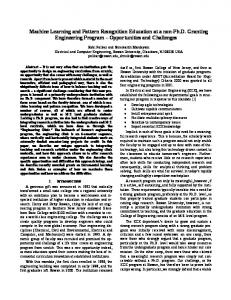
[23] Thus, apart from the addition of the positive constant m to the diagonal, the matrix system is identical to that for exact interpolation given by equation (9). This system can be converted to a positive definite form [Billings, 1998] and therefore always has a solution. [24] In summary, we select the value of m which gives the minimum value of G; m is then substituted into equation (14) which can in turn be solved for the TPS weights (L) and the polynomial coefficients (a). Once these have been obtained, equation (6) can be used to calculate the smoothed, interpolated AP misfit at any potential hypocenter. [25] The TPS surface, smoothed by the application of GCV (which is hereinafter called the misfit surface) of the points in Figure 1, is shown in Figure 3, and the effect of GCV is clear. Note how smooth the contours are once GCV has been applied and that the location of the minimum has not moved very much. The value of m in this case is 3.35 109. Typically, m lies between 109 and 108. Most importantly, there is only one minimum, and its location is closer to the EHB location (the center of Figure 3) once smoothing has been applied. Even when GCV is applied, it is possible for local minima to exist, but this is rather rare. Smoothing is effective in reducing the influence of random noise within the observational data. Conveniently, GCV automatically chooses a smoothing parameter based on a quantitative measure of the noise in the data. [26] As with other forms of smoothing, GCV does not reduce the effects of some systematic errors. The most important form of systematic error that can influence the AP locations is a systematic shift in the locations of the database events. This is known to occur in regions where the seismic velocity is significantly faster, or slower, on one side of the distribution of events (e.g., subduction zones). Billings et al. [1994] showed that events in the Flores Sea, Indonesia, may be systematically dragged toward Australia as a result of fast ray paths to Australian stations relative to the iasp91 reference model. Only low-magnitude events (mb < 4.5) were affected because higher-magnitude events were recorded at a large number and wide range of stations. The EHB catalogue contains few events of magnitude 4.5 or less, so it is unlikely that the AP results in this case will be strongly affected by systematic errors of this type. [27] Another source of systematic error is that a station may systematically record arrivals earlier, or later, due to


ESE

Figure 3. Contours of AP misfit at five depths for the same event as in Figures 1 and 2. In this case the thin-plate spline has been smoothed using generalized cross validation (see text). Notice that the contours are much simpler than in the unsmoothed case (Figure 2) and that the minimum, marked with a solid triangle, is closer to the EHB location (marked with a plus).

5-7

ESE

5-8


biased picking of arrival times or flaws in the timing of the data [e.g., Rohm et al., 1999]. If this form of bias is stationary over time, it has no effect on the AP method because the bias is present in the arrivals of both the new event and the database events, and so it cancels out in equation (2). In this case the AP method would perform the same job as station corrections in a standard least squares location method. However, systematic error in arrival times may change over time so the database should include events from a similar date to the new event if possible. [28] In all our examples using the EHB catalogue all comparable events within 200 km of the EHB location of the new event are used in the calculation of the misfit surface. This value is chosen to be certain that the real hypocentral location is contained in the region sampled. A larger volume could be used, but the calculation of the misfit surface becomes time consuming once the number of database points exceeds a few thousand. The determination of an AP hypocenter is computationally efficient provided there are less than 2000 nearby comparable events. Typically, 500 database events were used in the calculation of the misfit surface, and the AP hypocenter was found in 5 s on a Compaq XP1000 (500 MHz, specfp95 = 52.2). When the number of nearby comparable events is very large, the calculation of the GCV smoothing parameter, which scales as the cube of the number of comparable events, is the most expensive step. In our studies, using the EHB catalogue, the calculation of the AP hypocenter always took 10 km, the database events will tend to move out of their true depth layer (see Figure 5). Therefore this level of noise is significant in relation to the scale of the heterogeneities in the velocity model. The travel times of both the database events and the new events are assumed free from noise. [36] Figure 6 shows the median mislocations in the new events as a function of the mislocation in the database events. The AP locations have a smaller median error than the errors in the database events for a large range of database errors. We note that this range, extending from 2 to 60 km, spans the range of the noise often quoted in the real, teleseismic earthquake location problem. The first two circles are above the equality line, but the remainder lie below it. Interestingly, the AP locations actually improve once some noise is added. We believe that when there is no noise, there is no GCV smoothing and the minimum of the misfit surface tends to be drawn toward the most similar database event. As noise is added, the smoothing is more effective, and the locations are no longer pulled toward the


ESE

Figure 4. Similar to Figure 3 for an event a magnitude mb = 4.6 event in 1995. In this case the misfit ‘‘surface’’ is more complex, but the minimum is still well defined.

5-9

ESE

5 - 10


Figure 5. Synthetic layered Earth model. The arrows point from the original database locations to the locations once noise has been added. Note that many of the database events lie in the wrong layer once noise has been added.

database events. When the database noise is very large, the new events near the outside of the database distribution cannot be located using the AP method because the misfit surface for these events is very smooth and no longer has a minimum. In this example, a significant portion of the events cannot be located once the database error has a median of 60 km or more. [37] Figures 7a and 7b show the distributions of added noise for both the lateral and depth coordinates when noise with a standard deviation of 10 km is added. The database events used and the errors associated with this noise are shown in Figure 5. In this case, most of the database events are no longer in their correct velocity layer. The resulting errors in the AP locations are shown in Figures 7c and 7d. Clearly, the error in the AP locations is smaller (median error of 2.6 km laterally, 6.0 km in depth) than the errors in the database locations (7.1 km laterally and in depth) in both directions, which is contrary to the original postulate. Note that the mislocation in the lateral coordinate is smaller than in depth because of the geometry of the stations. We must conclude that GCV smoothing is successfully reducing the effects of the noise in the database events while retaining the significant signal. [38] This simple example shows that it is possible to extract useful information from a mislocated database to perform event location using the AP misfit measure equa-

Figure 6. Error in the AP locations as a function of noise added to the database locations. The dashed line represents equality between database error and AP error. The AP errors are smaller than the database errors over a large range.


ESE

5 - 11

Figure 7. Example of errors in the database locations and the resulting errors in the AP locations. In this case noise of standard deviation 10 km is added to both the lateral coordinate and depth. (a) Lateral and (b) depth errors and (c) lateral and (d) depth errors for the relocated events. Note that Figures 7c and 7d have smaller standard deviations than Figures 7a and 7b.

tion (1). Furthermore, the errors in the resulting locations can be smaller than those in the original database, even when we have the added problem of potential phase misidentification. This is due to the action of the GCV smoothing, which is successfully reducing the effects of the noise in the database events while retaining the significant signal. 2.6. Relocation of Ground Truth Events [39] To test the AP method against a standard location procedure using a 1-D Earth model, we relocated 395 nuclear blasts from the Nevada Test Site. This is a subset of the Prototype International Data Centers ground truth 0 events with a maximum error of 0.5 km determined from independent information [Bondar et al., 2001]. Sixty percent of the observations were teleseismic, and there were an average of 67 P, 18 Pn, and 6 PKP phases per event. Each event was also located using a standard misfit function measuring the discrepancies of observed arrivals and those

predicted from ak135 [Kennett et al., 1995]. The optimization of the misfit function was performed by the direct search neighborhood algorithm approach of Sambridge and Kennett [2001]. [40] In the application of the AP method we used the ground truth locations as the database, and the event being located was excluded. Events that lie near the outside of the database distribution can be difficult to locate using the AP method since the misfit surface may not have a welldefined minimum. This edge effect must be considered when the database does not completely cover the region of interest. It may be removed by adding artificial database events around the database distribution. These artificial events have travel times which are calculated from ak135 and the misfit value at the best database event is added to their misfit to simulate noise. In this case, 16 artificial events were added, 2 at each of the corners of a cube of side 200 km. The position of the cube is different for each new event, and it is centered on the database event with

ESE

5 - 12


Figure 8. Errors in ground truth locations when relocated using (a and b) the ak135 model, (c and d) AP method with ground truth database, and (e and f ) AP method using locations in Figures 8a and 8b as the database. The AP errors for both databases (Figures 8c, 8d, 8e, and 8f ) are smaller than the conventionally located database (Figures 8a and 8b).

NICHOLSON ET AL.: HYPOCENTER LOCATION BY PATTERN RECOGNITION Table 1. Mislocations in Ground Truth Events

Mean epicentral error, km Mean depth error, km

ak135 Locations

AP Locations With Ground Truth Database

AP Locations With ak135 Database

13.22 31.71

6.22 1.91

9.53 21.97

the lowest misfit to ensure the AP locations are not biased toward the ground truth location. We have found that changing the size of the cube has little effect on the AP locations. [41] The results are shown in Figure 8 and Table 1. They indicate that the AP locations are significantly better than the least squares locations, particularly in depth. Over 70% of the AP relocations are within 1 km of the ground truth depths. This example illustrates how good the AP locations can be when a very accurate database is available. Unlike the least squares locations, the AP locations are more accurate in depth than in epicenter, which is a result of

ESE

5 - 13

the ground truth locations being more densely grouped in depth than in epicenter. [42] As a further test we also applied the AP method to relocate the blasts, using the least squares locations shown in Figure 8a as the database. The results are summarized in Figure 8e and Table 1. The locations calculated using this database are significantly worse than when the ground truth locations were used. However, they are an improvement on the least squares locations on which they are based. The errors in depth increase dramatically due to the large errors in the database depths. However, the AP errors are still smaller than the database errors, demonstrating that as in the synthetic layered Earth considered in section 2.5, the AP locations can improve upon the database locations. In this case, both the AP locations and least squares locations experienced a systematic shift which increased as the number of observations decreased. When more than 200 observations were used, the least squares locations were 2.6 km NNE and AP locations were 3.8 km NE of the ground truth locations on average. When fewer than 100 observations are available, the systematic error in

Figure 9. Distance between EHB catalogue locations and AP locations for 500 events chosen randomly from the EHB catalogue. The median differences were 16.0 km in epicenter and 8.6 km in depth. These differences are only slightly larger than the error estimates given by EHB.

ESE

5 - 14


Figure 10. AP locations of 457 Atlantic Ocean events from the EHB catalogue: (a) the EHB locations and (b) the AP locations. Note how similar the two distributions are (see text for further discussion).

the ak135 locations is almost 4 times bigger at 10.3 km east of the real locations. However, the AP locations are not as badly affected, only increasing to 6.6 km NE of the ground truth locations. We suggest that this is due to the larger database events ‘‘anchoring’’ the distribution of AP locations. [43] We also tried using the EHB catalogue as the database with events from the test region removed. However, this left very few nearby database events, and AP locations could often not be made. Clearly, the AP method is only viable when the number of nearby database events is sufficient. When these conditions are satisfied, the relocation of ground truth events has been very successful. 2.7. Arrival Pattern Location Results for the EHB Catalogue [44] We have relocated 500 randomly chosen events from the EHB catalogue using the remainder of the EHB catalogue as the database. For each event the AP misfit was calculated for all database events within 250 km

of the EHB location. If there were