I - Pb - IEEE Xplore

ADAPTIV E BAYESIAN TRACKING WITH UNKNOWN TIME-VARYING SENSOR NETWORK PERFORMANCE

Giuseppe Papa*, Paolo Braca*, Steven Horn*, Stefano Marano+, Vincenzo Matta+ and Peter Willettt *

NATO STO CMRE, La Spezia, Italy, Email: {giuseppe.papalpaolo.bracalsteven.horn}@cmre.nato.int.

+

University of Salerno, Fisciano, Italy, Email: {marano/vmatta}@unisa.it.

t

University of Connecticut, Storrs CT, Email: [email protected].

A B S TRACT

In practical target tracking problems, the target detection perfor­ mance of the sensors may be unknown and may change rapidly with time. In this work we develop a target tracking procedure able to adapt and react to time-varying changes of the detection capability for a network of sensors. The proposed tracking strat­ egy is based on a Bayesian framework, in which the dynamic target state is augmented to include the sensor detection probabilities. The method is validated using computer simulations and real-world ex­ periments conducted by the NATO Science and Technology Organi­ zation (STO) - Centre for Maritime Research and Experimentation (CMRE). Index Terms- Multiple sensors, real-world data, Bayesian tar­ get tracking, particle filter, time-varying performance. 1. MOTIVATION A ND RELATED WORK

Multi-sensor target tracking is a challenging problem which involves data fusion of measurements from multiple sensors to perform joint detection and estimation of a moving object [1] . Measurements are usually subject to noise, missed detections, and false alarms. To cope with such non-idealities in the sensor model, the majority of target tracking algorithms assume the parameters which describe the sta­ tistical behaviour of the collected returns are known. However, in real-world applications these parameters may exhibit marked spatio­ temporal variations, and this will have a strong effect on the capabil­ ity of the tracking algorithms. A typical scenario is that of manoeuvring targets in which the behaviour of a target cannot be characterized at all times by a sin­ gle dynamic model and a solution should estimate on-line the proper dynamics assumed to model the target at the current time. The usual mechanism for this is often the interacting multiple model (IMM), see e.g. [2] . In several practical applications, a similar phenomenon can be observed for the performance of the sensors themselves, as opposed to the target dynamics. Now, in filtering problems the task of detecting - and sequestering - faulty sensors has been studied, see e.g. [3] ; however, in target tracking problems, even if the sensor is working correctly, its capability of observing a target can be affected by several factors, often difficult to characterize and model properly. Consider, for example, the degradation of detection capability when the target aspect is not favourable in terms of geometry with respect to the sensor, or when the signal-to-noise ratio (SNR) is completely unknown, see e.g. [4] . Another example is interference in backscat­ tered power due to the Bragg effect in HF surface wave radars [5] . In underwater sonar systems, target detections are influenced by sev­ eral environmental effects - for instance sound propagation - which

978-1-4673-6997-8/15/$31.00 ©2015 IEEE

have a strong dependence on unknown parameters (e.g. temperature, salinity, etc.) [6] that may change rapidly in time [7] . While a broad part of target tracking literature considers the sen­ sor performance to be a given, e.g. see [8, 9, 10, 11, 12, 13, 14, 15, 16, l7, 18] , and consequently the algorithm parameters perfectly matched to truth, only few recent papers focus on the problem of a mismatch of the sensor parameters, see [7, 4, 19, 20, 21] . The key aspect of this work is that the sensor detection capa­ bility of a target is not only unknown and spatially dependent, but that it may change rapidly in time. A target tracking procedure will be developed to adapt to the changes in the sensor detection capa­ bility. In particular, a full Bayesian framework is derived to model the behaviour of a network of sensors in which each sensor has its own time-varying detection capability. The dynamic target state is augmented to add the detection probabilities of each sensor in the network, and the dynamics of this detection probability are modeled as a time-varying Markov process. This proposed method is validated using both computer experi­ ments and real-world data collected during the CMRE HF-radar ex­ periment, which took place between May and December 2009 on the Ligurian coast of the Mediterranean Sea, see more details in [5] .

2. PROBLEM FORMALIZATION

Consider a system consisting of a network of Ns sensors, whose aim is to monitor a surveillance region. In particular, the aim is to detect target presence/absence and, in the case of presence, to track the target state. Without loss of generality we consider a two­ dimensional surveillance region with area V. At time scan k the target of interest can be present or absent. When the target is present, its state is Xk = [Pk ,Pk ,P% ,p%f, where Pk and p% are the position coordinates and Pk and p% are the velocities in the two dimensions. For ease of notation, we also define the set Xb where Xk = ° when the target is absent, otherwise Xk = {xk}. This is a compact representation of the target presence/absence and the target state. In the target tracking literature, see e.g. [22] , Xk is often referred to as a Bernoulli Random Finite Set (RFS) [9, 12, 15, 16, 17] . The time evolution of Xk is ruled by the distribution

2534

Pb , Pb fb (Xk) , 1 Ps , Ps f (xklxk-l),

{I

-

-

Xk = Xk = Xk = Xk =

0,Xk-1 = 0, {xk} ,Xk-1 = 0, 0,Xk-1 = {xk-d, {xk} ,Xk-1 = {xk-d,

(1)

ICASSP2015

where Pb and fb (x) are respectively the target birth probabil­ ity and the target birth distribution, while Ps and f (xklxk-l) are respectively the target survival probability and the target state transition distribution. The latter is often given by the relation Xk = Fk (Xk-l,Vk), where Fk is the state transition function (in general non-linear) and Vk is the process noise, often assumed as a sequence of independent and identically distributed (i.i.d.) random variables.

distinguish statistically between the case of target presence and ab­ sencel. Consequently, it is assumed that PI, cannot have values be­ Iow a given threshold P �i n > 0. Algorithm 1 Adaptive Tracker using particle filtering.

IMPORTANCE SAMPLING Draw

xt

Pt = 1 to N do

Draw

for

2.1. Measurement origin uncertainty

Nn

xk from U

(x; z'k,i )

end for

w

(2)

� =C(ZkIXk = 0) [(1- Pb)wL 1 + (l-ps ) (1- W L1 ) ] ; with the lowest

Nn NZk

weights;

NORMALIZATION Np

Wt =w �

+

2: wk; { Total weight }

j=l

Wki - w� Wt.

(� ) -1

'

1

"tj'� = , ... , Np;

RESAMPLI G

(3)

i w"k 2

Ne!! =

where hs is the measurement function and Wk is an i.i.d. measure­ ment noise sequence. If the target is detected by the sensor, then

if Ne!!

J=l


0, zEZ;; 1Jc (Zk) = M(O;A") , mk =0,

(5)

where M(m;AS) and AS are respectively the distribution and the av­ erage number of clutter elements, while CS ( z ) is the PDF of a clutter element. Often, M(m;AS) is assumed to be Poisson and CS(z) uni­ form [18, 6] . It is possible to show that the likelihood for the sensor s, when the target is present, is given by

P (Zkl{xd,Pk) = ( 1 - Pk) 1Jc (Zk) + + P k L f (ZIXk) 1Jc (Zk\Z)

In real-world applications, the detection performance of a sensor Pk is usually time-varying and spatially-varying, because it depends on environmental conditions, aspect, interference, etc. (see e.g. [7, 5, 6] ). Now, it is noted that the likelihood (6) is strongly dependent on the sensor detection probabilities, and, consequently, a sequential Bayesian procedure is proposed in which the detection probabilities are included in the dynamic system state. The state at time k is then redefined as Xk = {(Xk,Pk)}, when the target is present, while it remains Xk = 0, when the target it absent. The posterior distribu­ tion given all the measurements up to time scan k is given by

P(XkIZl.k where Zlk (5)-(6)

d!l

)

=

qZkIXk)P(XkIZlk -1) , P (ZkIZlk-1)

{Zl"'" Zk}

and.c

(ZkIXk) is given by eq. (4)­

Ns

qZkl0) = IT P(Z'k10) , 8=1

(8)

Ns

(6)

qZkl {(Xk,Pk)}) = IT P(Zkl {xd ,Pk) ' 8=1

zEZk

It is worth noting that when PI, = ° (target present but not observ­ able), the likelihoods (5) and (6) coincide and it is not possible to

(7)

I

This work considers the case of target not present and target not observ­

able to be the same case.

2535

(9)

-50

Ground truth _Adaptive tracker -+-Non-adaptive tracker

-52

-3

-54

-4

-56

-5

� -58

I

;" -60

�

-6

-62 -7

-64

-8

-66 -54

-52

-50

-48

-46

-44 x

(a)

[km[

-42

-40

-38

-36

-34

5 x

HFSW radar tracks and ground-truth (AlS). � Non-adaptive - K

tracker Adaptive tracker - s =

- Adaptive tracker -

�

8 =

[km[

6

(a) Tracks generated using simulated data.

-Ground truth -+- Non-adaptive tracker � Adaptive tracker - s = - M - Adaptive tracker - s =

1 2

1 2

go.s :0 " oD

2

0.6

.g S Cl

0.4

0.. =

0.2

0.2

�0----� 5�0 ----�60' °0L---�'0�--�20�--�30-----4 k

0 � ----� 5�0----�60 °0�--�'�0 ----�20�--�30-----4 k

(b) Time-varying detection probability profile.

(b) Time-varying detection probability profile.

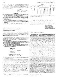
Fig. 1. Comparison between the adaptive and non-adaptive tracker

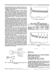
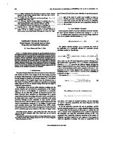
Fig. 2. Comparison between the adaptive and non-adaptive tracker

using the dataset of two HFSW radar systems (WERA). Panel (a) presents the trajectories, when the target is declared as present, and the ground-truth given by the AIS messages. Panel (b) presents the value of the detection probability, constant and fixed to 0.9 for the non-adaptive tracker, while for the adaptive tracker the mode of the posterior distribution of the detection probability for the two sensors, s = 1,2, is shown.

using simulated data. In panel (a) the trajectories, when the target is declared as present, are reported. Panel (b) presents the value of the detection probability, constant and fixed to 0.9, for the non­ adaptive tracker, while for the adaptive tracker we report the mode of the posterior distribution of the detection probability for the two sensors, S = 1,2. An abrupt change in the true detection probability is simulated at the time scan k = 30.

The prediction term can be written as

where each f; (PkIPk-l,Xk) is the transition distribution of the cor­ responding Pk of the sensor s.

P (XkIZlk-l) = x(XkI0)P (0IZlk-l) + +

!! x (Xkl {(x,p)})P ({(x,p)} IZlk-l)dxdp,

3.1. Particle filter implementation

the RFS transition distribution for the augmented state is indicated with x (XkIXk-1). Note that this distribution has the same structure of eq. (1). There are two functions to be defined: the birth distribution fb (Xk' Pk); and the state transition distribution fx,p (Xk' PkIXk-l,Pk-l). This latter can be recast as

Since a closed form for (7) is hard (or even impossible) to derive, a numerical implementation of the filter based on the Sequential Monte Carlo methods [23] applied to RFS [24] is employed. The posterior distribution at time scan k (7) is represented by

fx,p (Xk,Pklxk-l,Pk-l) = f (xklxk-l) fp (pklpk-l,Xk)' where fp (PkIPk-l,Xk) is the detection probability transition distri­

bution, formally dependent from the target state ( e.g. the geometry target-sensor). Assuming that the sensors are conditionally indepen­ dent, the detection probability transition distribution is given by Ns

fp(Pklpk-l,Xk) = IIf; (Pklpk-l,xk), s=l

(10)

Xk = {(x,p)} , where

w� is the weight approximating P (Xk

=

(11)

0IZlk), (xl,pt)

is the i-th sample of the augmented system state, Wk is the i-th weight approximating P (Xk = {(xl,Pk)} IZlk), Np is the num­ ber of particles.

2536

Par.

Algorithm I presents the pseudo-code of the particle filter im­ plementation for the augmented sequential Bayesian filter, referred as the adaptive tracker. Note that the resampling algorithm is stan­ dard and given in [23] . The initial samples Xo are uniformly drawn in the surveillance area for the positional coordinates and in [ -Vmax, Vmax 1 for the speed coordinates, while the initial samples Po are uniformly drawn in rh x ... x nN where ns is the support of the detection proba­ bility distribution. For instance, assuming a continuous distribution the support is defined as ns = [P�in' 1]. The initial weights Wo

T av aT a

Np Pb Ps Ns Nn

s'

w2

= 0.5. In the importance are all initialized to (2Np)-\ while sampling step of the filter, two kinds of importance sampling distri­ butions are used. The first one is the augmented system state tran­ sition distribution and is used to predict the new samples (xl,pt), Vi = 1, . . . ,Np, from the Np samples at the previous step. The sec­ ond one is constructed on the basis of the measurements Zk and can be interpreted as the target birth distribution. For each measurement z E Zk' Vs, Nn particles (xL Pt) are sampled, where Xk is drawn from U (x; z ) , which is the uniform distribution in [ -Vmax, Vmax] for the speed coordinates and centered in z with a given width for the position coordinates, and Pk is drawn from U (p), which is a uniform distribution in 0,1 x ... x nN . The total number of new particles is NnNzk, where NZk = L:� l IZk l.

4. EXPERIMENTAL RESULTS

This section reports the results of the adaptive tracker, using both computer simulated experiments and real-world data collected dur­ ing the CMRE HF-radar experiment, see details in [5] . Two Wellen radar (WERA) systems were deployed on the Italian coast of the Ligurian Sea, one on Palmaria island near La Spezia (44° 2' 30/1 N, go 50' 36/1 E) and the other at San Rossore Park near Pisa (43° 40' 53/1 N, 10° 16' 52/1 E). The target state is defined in Cartesian coordinates, with a fixed origin located at the Palmaria radar site. Consider the real track of a vessel sailing North-West, as re­ ported by the data transmitted by its Automatic Identification Sys­ tem (AIS) transponder. The AIS track positions, based on GPS, are referred to here as the ground-truth, see also the discussion in [5] . Figure I(a) reports the tracks generated by the proposed adaptive tracking procedure and the non-adaptive one with fixed detection probabilities for both the sensors. The parameters of the algorithms are reported in Tab. 1. Note that all of the parameters of each of the algorithms are identical, including the number of particles, even though state augmentation should require, in theory, a larger num­ ber of particles. The only difference is in the use of the detection probability (fixed for the non-adaptive tracker). The presence or absence of the target at each frame is decided based on the value of the marginal posterior probability P (0IZ lk), and if, for instance, this probability exceeds a given threshold then the target absence is declared. In the scenario reported in Figure I it is easy to verify that the target trajectory is completely reconstructed by the adaptive tracker while the non-adaptive tracker exhibits some "gaps " in the estimated track. This phenomenon seems to be caused by abrupt decreases of the detection probability in one (or both) of the two radars with respect to the nominal values, these calibrated and fixed to 0.9 for the non-adaptive tracker. Calibrating the values for a non-adaptive tracker is often an ad-hoc process, or possibly as a calibration of static parameters [5] . It is worthwhile to note that the adaptive tracker has the ability to follow these apparent oscil­ lations in detection probability, see Figure I(b), resulting in better track hold. For the sake of further clarity, this phenomenon is also reconstructed using synthetic data.

b

A/V

Td

I

I

Simulation

40s 5 10-3 m/ s2 75 m 1° 1.2 10-8 m-2 5 104 10-2 1 - 10-3 2 250 0.5

HFSW Radar

33.28 s 5 10-3 m/ s2 75 m 1° 2 10-9 m-2 5 104 10-4 1 - 10-4 2 250 0.5

I

Specification Time scan Process noise st. dev. Range st. dev. Bearing st. dev. Clutter density Number of particles Birth probability Survival probability Number of sensors Particles per meas. Degeneracy threshold

Table 1. Parameter values used in in the algorithm for simulated and

real radar data.

Consider the scenario reported in Figure 2, in which the target is sailing North-West. The data are generated using the MOU model, described in Sec. 2.1 and with the parameters reported in Tab. I, with the true value of the detection probability for both the sensors fixed at 0.9 in first 30 scans followed by an abrupt decrease to 0.3. This simulates such phenomena as unfavorable propagation, interference or a change in the target aspect geometry - all commonly observed in target tracking applications, as discussed. In the simulation, the non-adaptive tracker uses a detection prob­ ability fixed at 0.9 for both the sensors. It is easy to verify from Fig­ ure 2(a) that after 30 scans the non-adaptive tracker fails to maintain hold of the target track. The adaptive tracker, instead, is able to also track the abrupt change in the detection probability without losing the target, i.e. correctly declaring that the target is present. In the two examples presented here one way to evaluate the over­ all detection performance of the trackers is using the time-on-target (ToT) metric, see e.g. [5] . Another option, not presented here, would be to compute the OSPA metric [25] . The ToT for the adaptive tracker is 100%, whereas for the non-adaptive is 60% and 63% for the HFSW radar dataset and the simulated dataset, respectively. 5. CONCLUSIONS

This paper presented a target tracking procedure, developed for a network of sensors, which is able to adapt and react to the time­ varying changes of the sensors target detection capability. The pro­ posed tracking strategy is based on a Bayesian framework, and the implementation of the tracker is based on the particle filtering ap­ proach for the RFS, however, the dynamic target state is augmented with the addition of sensor detection probabilities. The method was validated using computer simulations and real­ world experiments, conducted by the NATO Science and Technol­ ogy Organization (STO) - Centre for Maritime Research and Exper­ imentation (CMRE). At the cost of some computational complexity in the particle update, with no additional cost in number of particles, it was shown that the ToT metric was greatly improved over the non­ adaptive tracking approach. This shows a significant benefit in the use of the adaptive tracker achieving a ToT of 100% vice roughly 60% for the non-adaptive tracker. 6. ACKNOWLEDGEMENTS

This work has been funded by the NATO Allied Command Transfor­ mation (NATO-ACT) under the project Maritime Situational Aware­ ness.

2537

7. REFERENCES

[1] Y. Bar-Shalom, P. Willett, and X. Tian, Tracking and Data Fusion: A Handbook of Algorithms, YBS Publishing, Storrs, CT, 2011. [2] E. Mazor, A. Averbuch, , Y. Barshalom, and J. Dayan, "Inter­ acting multiple model methods in target tracking: A survey, " IEEE Trans. Aerosp. Electron. Syst., vol. 34, no. 1, pp. 103123, Jan. 1998.

[14] P. Braca, M. Guernero, S. Marano, Y. Matta, and P. Willett, "Selective measurement transmission in distributed estimation with data association, " IEEE Trans. Signal Process., vol. 58, no. 8, pp. 4311-4321, Aug. 2010. [15] P. Braca, S. Marano, Y. Matta, and P. Willett, "Multitarget­ multisensor ML and PHD: Some asymptotics, " in Proc. of the 15th Intern. Con! on Inform. Fusion (FUSION), Singapore, 2012.

[3] M. Basseville and I. Y. Nikiforov, Detection of Abrupt Changes: T heory and Application, Prentice-Hall, Englewood Cliffs, NJ, 1993.

[16] P. Braca, S. Marano, Y. Matta, and P. Willett, "Asymptotic efficiency of the PHD in multitarget/multisensor estimation, " IEEE 1. Sel. Topics Signal Process., vol. 7, no. 3, pp. 553-564, June 2013.

[4] D. Clark, B. Ristic, Ba-Ngu Vo, and Ba-Tuong Vo, "Bayesian multi-object filtering with amplitude feature likelihood for un­ known object SNR, " IEEE Trans. Signal Process., vol. 58, no. l, pp. 26-37, Jan. 2010.

[17] P. Braca, S. Marano, Y. Matta, and P. Willett, "A linear complexity particle approach to the exact multi-sensor PHD, " in in Proc. IEEE Int. Con/. Acoust., Speech, Signal Process. (ICASSP), May 2013.

[5] S. Maresca, P. Braca, J. Horstmann, and R. Grasso, "Mar­ itime surveillance using multiple high-frequency surface-wave radars, " IEEE Trans. Geosci. Remote Sens., vol. 52, no. 8, pp. 5056-5071, Aug. 2014. [6] P. Braca, P. Willett, K. LePage, S. Marano, and Y. Matta, "Bayesian tracking in underwater wireless sensor networks with port-starboard ambiguity, " IEEE Trans. Signal Process., vol. 62, no. 7, pp. 1864-1878, Apr. 2014.

[18] P. Braca, R. Goldhahn, K. LePage, P. Willett, S. Marano, and Y. Matta, "Cognitive multistatic auv networks, " in Proc. of the 17th Intern. Con! on Inform. Fusion (FUSION), Salamanca, 2014. [19] R. Mahler, Ba-Thong Vo, and Ba-Ngu Vo, "CPHD filtering with unknown clutter rate and detection profile, " Signal Pro­ cessing, IEEE Transactions on, vol. 59, no. 8, pp. 3497-3513, Aug. 2011.

[7] W. Blanding, P. Willett, Y. Bar-Shalom, and S. Coraluppi, "Multisensor track management for targets with fluctuating SNR, " IEEE Trans. Aerosp. Electron. Syst., vol. 45, no. 4, pp. 1275-1292, Oct. 2009.

[20] Ba-Thong Vo, Ba-Ngu Vo, R. Hoseinnezhad, and R. Mahler, "Robust multi-bernoulli filtering, " IEEE 1. Sel. Topics Signal Process., vol. 7, no. 3, pp. 399-409, June 2013.

[8] S. Coraluppi and D. Grimmett, "Multistatic sonar tracking, " in Proc. of SPIE Conference on Signal Processing, Sensor Fu­ sion, and Target Recognition XII, Orlando FL, USA, Apr. 2003.

[21] B. Ristic, D. Clark, Ba-Ngu Vo, and Ba-Thong Vo, "Adaptive target birth intensity for PHD and CPHD filters, " IEEE Trans. Aerosp. Electron. Syst., vol. 48, no. 2, pp. 1656-1668, Apr. 2012.

[9] R. Mahler, "Multitarget Bayes filtering via first-order multi­ target moments, " IEEE Trans. Aerosp. Electron. Syst., vol. 39, no. 4, pp. 1152-1178, Jan. 2003. [10] C. Kreucher, A.O. Hero, and K. Kastella, "A comparison of task driven and information driven sensor management for tar­ get tracking, " in 44th IEEE Con! on Decision and Control, 2005 and 2005 European Control Conference (CDC-ECC), 2005. [11] M. R. Morelande, C. M. Kreucher, and K. Kastella, "A Bayesian approach to multiple target detection and tracking, " IEEE Trans. Signal Process., vol. 55, no. 5, pp. 1589-1604, May 2007. [12] Ba-Tuong Vo, Ba-Ngu Vo, and A. Cantoni, "Bayesian filter­ ing with random finite set observations, " IEEE Trans. Signal Process., vol. 56, no. 4, pp. 1313-1326, Apr. 2008. [13] O. Erdinc, P. Willett, and Y. Bar-Shalom, "The bin-occupancy filter and its connection to the PHD filters, " IEEE Trans. Signal Process., vol. 57, no. 11, pp. 4232-4246, Nov. 2009.

[22] B. Ristic, Ba-Thong Vo, Ba-Ngu Vo, and A. Farina, "A tutorial on Bernoulli filters: Theory, implementation and applications, " IEEE Trans. Signal Process., vol. 61, no. 13, pp. 3406-3430, July 2013. [23] M.S. Arulampalam, S. Maskell, N. Gordon, and T. Clapp, "A tutorial on particle filters for online nonlinear/non-Gaussian Bayesian tracking, " IEEE Trans. Signal Process., vol. 50, no. 2, pp. 174 -188, Feb. 2002. [24] B.-N. Vo, S. Singh, and A. Doucet, "Sequential Monte Carlo methods for multitarget filtering with random finite sets, " IEEE Trans. Aerosp. Electron. Syst., vol. 41, no. 4, pp. 1224-1245, Oct. 2005. [25] D. Schuhmacher, B.-T. Vo, and B.-N. Vo, "A consistent met­ ric for performance evaluation of multi-object filters, " IEEE Trans. Signal Process., vol. 56, no. 8, pp. 3447-3457, Aug. 2008.

2538