i2MapReduce: Incremental MapReduce for Mining Evolving Big Data

i2 MapReduce: Incremental MapReduce for Mining Evolving Big Data Yanfeng Zhang

Shimin Chen

Qiang Wang

Northeastern University, China

Institute of Computing Technology, CAS

Northeastern University, China

[email protected]

[email protected] Ge Yu

[email protected]

arXiv:1501.04854v1 [cs.DC] 20 Jan 2015

Northeastern University, China

[email protected] ABSTRACT As new data and updates are constantly arriving, the results of data mining applications become stale and obsolete over time. Incremental processing is a promising approach to refreshing mining results. It utilizes previously saved states to avoid the expense of re-computation from scratch. In this paper, we propose i2 MapReduce, a novel incremental processing extension to MapReduce, the most widely used framework for mining big data. Compared with the state-of-the-art work on Incoop, i2 MapReduce (i) performs key-value pair level incremental processing rather than task level re-computation, (ii) supports not only one-step computation but also more sophisticated iterative computation, which is widely used in data mining applications, and (iii) incorporates a set of novel techniques to reduce I/O overhead for accessing preserved fine-grain computation states. We evaluate i2 MapReduce using a one-step algorithm and three iterative algorithms with diverse computation characteristics. Experimental results on Amazon EC2 show significant performance improvements of i2 MapReduce compared to both plain and iterative MapReduce performing re-computation.

1.

INTRODUCTION

Today huge amount of digital data is being accumulated in many important areas, including e-commerce, social network, finance, health care, education, and environment. It has become increasingly popular to mine such big data in order to gain insights to help business decisions or to provide better personalized, higher quality services. In recent years, a large number of computing frameworks [9, 25, 23, 18, 19, 17, 11, 7, 10, 28] have been developed for big data analysis. Among these frameworks, MapReduce [9] (with its open-source implementations, such as Hadoop) is the most widely used in production because of its simplicity, generality, and maturity. We focus on improving MapReduce in this paper.

Permission to make digital or hard copies of all or part of this work for personal or classroom use is granted without fee provided that copies are not made or distributed for profit or commercial advantage and that copies bear this notice and the full citation on the first page. Copyrights for components of this work owned by others than ACM must be honored. Abstracting with credit is permitted. To copy otherwise, or republish, to post on servers or to redistribute to lists, requires prior specific permission and/or a fee. Request permissions from [email protected]. Copyright 20XX ACM X-XXXXX-XX-X/XX/XX ...$15.00.

Big data is constantly evolving. As new data and updates are being collected, the input data of a big data mining algorithm will gradually change, and the computed results will become stale and obsolete over time. In many situations, it is desirable to periodically refresh the mining computation in order to keep the mining results up-to-date. For example, the PageRank algorithm [5] computes ranking scores of web pages based on the web graph structure for supporting web search. However, the web graph structure is constantly evolving; Web pages and hyper-links are created, deleted, and updated. As the underlying web graph evolves, the PageRank ranking results gradually become stale, potentially lowering the quality of web search. Therefore, it is desirable to refresh the PageRank computation regularly. Incremental processing is a promising approach to refreshing mining results. Given the size of the input big data, it is often very expensive to rerun the entire computation from scratch. Incremental processing exploits the fact that the input data of two subsequent computations A and B are similar. Only a very small fraction of the input data has changed. The idea is to save states in computation A, re-use A’s states in computation B, and perform re-computation only for states that are affected by the changed input data. In this paper, we investigate the realization of this principle in the context of the MapReduce computing framework. A number of previous studies (including Percolator [22], CBP [16], and Naiad [20]) have followed this principle and designed new programming models to support incremental processing. Unfortunately, the new programming models (BigTable observers in Percolator, stateful translate operators in CBP, and timely dataflow paradigm in Naiad) are drastically different from MapReduce, requiring programmers to completely re-implement their algorithms. On the other hand, Incoop [4] extends MapReduce to support incremental processing. However, it has two main limitations. First, Incoop supports only task-level incremental processing. That is, it saves and reuses states at the granularity of individual Map and Reduce tasks. Each task typically processes a large number of key-value pairs (kvpairs). If Incoop detects any data changes in the input of a task, it will rerun the entire task. While this approach easily leverages existing MapReduce features for state savings, it may incur a large amount of redundant computation if only a small fraction of kv-pairs have changed in a task. Second, Incoop supports only one-step computation, while important mining algorithms, such as PageRank, require iterative computation. Incoop would treat each iteration as a separate MapReduce job. However, a small number of in-

put data changes may gradually propagate to affect a large portion of intermediate states after a number of iterations, resulting in expensive global re-computation afterwards. We propose i2 MapReduce, an extension to MapReduce that supports fine-grain incremental processing for both onestep and iterative computation. Compared to previous solutions, i2 MapReduce incorporates the following three novel features: • Fine-grain Incremental Processing using MRBGStore: Unlike Incoop, i2 MapReduce supports kv-pair level fine-grain incremental processing in order to minimize the amount of re-computation as much as possible. We model the kv-pair level data flow and data dependence in a MapReduce computation as a bipartite graph, called MRBGraph. A MRBG-Store is designed to preserve the fine-grain states in the MRBGraph and support efficient queries to retrieve fine-grain states for incremental processing. (cf. Section 3) • General-Purpose Iterative Computation with Modest Extension to MapReduce API: Our previous work proposed iMapReduce [28] to efficiently support iterative computation on the MapReduce platform. However, it targets types of iterative computation where there is a oneto-one/all-to-one correspondence from Reduce output to Map input. In comparison, our current proposal provides general-purpose support, including not only one-to-one, but also one-to-many, many-to-one, and many-to-many correspondence. We enhance the Map API to allow users to easily express loop-invariant structure data, and we propose a Project API function to express the correspondence from Reduce to Map. While users need to slightly modify their algorithms in order to take full advantage of i2 MapReduce, such modification is modest compared to the effort to re-implement algorithms on a completely different programming paradigm, such as in Percolator [22], CBP [16], and Naiad [20]. (cf. Section 4) • Incremental Processing for Iterative Computation: Incremental iterative processing is substantially more challenging than incremental one-step processing because even a small number of updates may propagate to affect a large portion of intermediate states after a number of iterations. To address this problem, we propose to reuse the converged state from the previous computation and employ a change propagation control mechanism. We also enhance the MRBG-Store to better support the access patterns in incremental iterative processing. To our knowledge, i2 MapReduce is the first MapReduce-based solution that efficiently supports incremental iterative computation. (cf. Section 5) We implemented i2 MapReduce by modifying Hadoop-1.0.3. We evaluate i2 MapReduce using a one-step algorithm (APriori) and three iterative algorithms (PageRank, Kmeans, GIM-V) with diverse computation characteristics. Experimental results on Amazon EC2 show significant performance improvements of i2 MapReduce compared to both plain and iterative MapReduce performing re-computation. For example, for the iterative PageRank computation with 10% data changed, i2 MapReduce improves the run time of recomputation on plain MapReduce by a 8 fold speedup. (cf. Section 8)

2.

MAPREDUCE BACKGROUND

Input Data Blocks



Map

Reduce Final Results

Map

Reduce

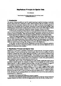
Figure 1: MapReduce computation. A MapReduce program is composed of a Map function and a Reduce function [9], as shown in Fig. 1. Their APIs are as follows: map(K1, V 1) → [hK2, V 2i] reduce(K2, {V 2}) → [hK3, V 3i] The Map function takes a kv-pair hK1, V 1i as input and computes zero or more intermediate kv-pairs hK2, V 2is. Then all hK2, V 2is are grouped by K2. The Reduce function takes a K2 and a list of {V 2} as input and computes the final output kv-pairs hK3, V 3is. A MapReduce system (e.g., Apache Hadoop) usually reads the input data of the MapReduce computation from and writes the final results to a distributed file system (e.g., HDFS), which divides a file into equal-sized (e.g., 64MB) blocks and stores the blocks across a cluster of machines. For a MapReduce program, the MapReduce system runs a JobTracker process on a master node to monitor the job progress, and a set of TaskTracker processes on worker nodes to perform the actual Map and Reduce tasks. The JobTracker starts a Map task per data block, and typically assigns it to the TaskTracker on the machine that holds the corresponding data block in order to minimize communication overhead. Each Map task calls the Map function for every input hK1, V 1i, and stores the intermediate kv-pairs hK2, V 2is on local disks. Intermediate results are shuffled to Reduce tasks according to a partition function (e.g., a hash function) on K2. After a Reduce task obtains and merges intermediate results from all Map Tasks, it invokes the Reduce function on each hK2, {V 2}i to generate the final output kv-pairs hK3, V 3is.

3. FINE-GRAIN INCREMENTAL PROCESSING FOR ONE-STEP COMPUTATION We begin by describing the basic idea of fine-grain incremental processing in Section 3.1. In Section 3.2–3.3, we present the main design, including the MRBGraph abstraction and the incremental processing engine. Then in Section 3.4–3.5, we delve into two aspects of the design, i.e. the mechanism that preserves the fine-grain states, and the handling of a special but popular case where the Reduce function performs accumulation operations.

3.1 Basic Idea Consider two MapReduce jobs A and A′ performing the same computation on input data set D and D′ , respectively. D′ = D+∆D, where ∆D consists of the inserted and deleted input hK1, V 1is1 . An update can be represented as a dele1 We assume that new data or new updates are captured via incremental data acquisition or incremental crawling [8,

stance, (ii) the destination Reduce instance (as identified by K2), and (iii) the edge value (i.e. V 2). Since Map input key K1 may not be unique, i2 MapReduce generates a globally unique Map key M K for each Map instance. Therefore, i2 MapReduce will preserve (K2, M K, V 2) for each MRBGraph edge.

3.3 Fine-grain Incremental Processing Engine Fig. 3 illustrates the fine-grain incremental processing engine with an example application, which computes the sum of in-edge weights for each vertex in a graph. As shown at the top of Fig. 3, the input data, i.e. the graph structure, evolves over time. In the following, we describe how the engine performs incremental processing to refresh the analysis results. Figure 2: MRBGraph. tion followed by an insertion. Our goal is to re-compute only the Map and Reduce function call instances that are affected by ∆D. Incremental computation for Map is straightforward. We simply invoke the Map function for the inserted or deleted hK1, V 1is. Since the other input kv-pairs are not changed, their Map computation would remain the same. We now have computed the delta intermediate values, denoted ∆M , including inserted and deleted hK2, V 2is. To perform incremental Reduce computation, we need to save the fine-grain states of job A, denoted M , which includes hK2, {V 2}is. We will re-compute the Reduce function for each K2 in ∆M . The other K2 in M does not see any changed intermediate values and therefore would generate the same final result. For a K2 in ∆M , typically only a subset of the list of V 2 have changed. Here, we retrieve the saved hK2, {V 2}i from M , and apply the inserted and/or deleted values from ∆M to obtain an updated Reduce input. We then re-compute the Reduce function on this input to generate the changed final results hK3, V 3is. It is easy to see that results generated from this incremental computation are logically the same as the results from completely re-computing A′ .

3.2 MRBGraph Abstraction We use a MRBGraph (Map Reduce Bipartite Graph) abstraction to model the data flow in MapReduce, as shown in Fig. 2 (a). Each vertex in the Map task represents an individual Map function call instance on a pair of hK1, V 1i. Each vertex in the Reduce task represents an individual Reduce function call instance on a group of hK2, {V 2}i. An edge from a Map instance to a Reduce instance means that the Map instance generates a hK2, V 2i that is shuffled to become part of the input to the Reduce instance. For example, the input of Reduce instance a comes from Map instance 0, 2, and 4. MRBGraph edges are the fine-grain states M that we would like to preserve for incremental processing. An edge contains three pieces of information: (i) the source Map in21]. Incremental data acquisition can significantly save the resources for data collection; it does not re-capture the whole data set but only capture the revisions since the last time that data was captured.

Initial Run and MRBGraph Preserving. The initial run performs a normal MapReduce job, as shown in Fig. 3 (a). The Map input is the adjacency matrix of the graph. Every record corresponds to a vertex in the graph. K1 is vertex id i, and V 1 contains “j1 :wi,j1 ; j2 :wi,j2 ; . . . ” where j is a destination vertex and wi,j is the weight of the outedge (i, j). Given such a record, the Map function outputs intermediate kv-pair hj, wi,j i for every j. The shuffling phase groups the edge weights by the destination vertex. Then the Reduce function computes for a vertex j the sum of all its P in-edge weights as i wi,j . For incremental processing, we preserve the fine-grain MRBGraph edge states. A question arises: shall the states be preserved at the Map side or at the Reduce side? We choose the latter because during incremental processing original intermediate values can be obtained at the Reduce side without any shuffling overhead. The engine transfers the globally unique M K along with hK2, V 2i during the shuffle phase. Then it saves the states (K2, M K, V 2) in a MRBGraph file at every Reduce task, as shown in Fig. 2 (b). Delta Input. i2 MapReduce expects delta input data that contains the newly inserted, deleted, or modified kv-pairs as the input to incremental processing. Note that identifying the data changes is beyond the scope of this paper; Many incremental data acquisition or incremental crawling techniques have been developed to improve data collection performance [8, 21]. Fig. 3 (b) shows the delta input for the updated application graph. A ‘+’ symbol indicates a newly inserted kv-pair, while a ‘-’ symbol indicates a deleted kv-pair. An update is represented as a deletion followed by an insertion. For example, the deletion of vertex 1 and its edge are reflected as h1, 2:0.4,‘-’i. The insertion of vertex 3 and its edge leads to h3, 0:0.1,‘+’i. The modification of the vertex 0’s edges are reflected by a deletion of the old record h0, 1:0.3;2:0.3,‘-’i and an insertion of a new record h0, 2:0.6,‘-’i. Incremental Map Computation to Obtain the Delta MRBGraph. The engine invokes the Map function for every record in the delta input. For an insertion with ‘+’, its intermediate results hK2, M K, V 2′ is represent newly inserted edges in the MRBGraph. For a deletion with ‘-’, its intermediate results indicate that the corresponding edges have been removed from the MRBGraph. The engine replaces the V 2′ s of the deleted MRBGraph edges with ‘’. During the MapReduce shuffle phase, the intermediate hK2, M K, V 2′ is and hK2, M K,‘-’is with the same K2 will be grouped together. The delta MRBGraph will contain

Merge

Reduce

Index Read Cache

K2a K2b K2c ...

Main memory

Append Buffer

Chunk 0

Disk

(K2a, {MK*, V*,a})

K2b MK2 K2c MK7 V27,c ... Delta MRBGraph (from incremental processing)

Chunk 1 Read (K2b, {MK*, V*,b}) Window Chunk 2 (K2c, {MK*, V*,c})

…… MRBGraph File

MRBGStore

Figure 4: Structure of MRBG-Store.

Figure 3: Incremental processing for an application that computes the sum of in-edge weights for each vertex. only the changes to the MRBGraph and sorted by the K2 order. Incremental Reduce Computation. The engine merges the delta MRBGraph and the preserved MRBGraph to obtain the updated MRBGraph using the algorithm in Section 3.4. For each hK2, M K,‘-’i, the engine deletes the corresponding saved edge state. For each hK2, M K, V 2′ i, the engine first checks duplicates, and inserts the new edge if no duplicate exists, or else updates the old edge if duplicate exists. (Note that (K2,M K) uniquely identifies a MRBGraph edge.) Since an update in the Map input is represented as a deletion and an insertion, any modification to the intermediate edge state (e.g., h2, 0, ∗i in the example) consists of a deletion (e.g., h2, 0,‘-’i) followed by an insertion (e.g., h2, 0, 0.6i). For each affected K2, the merged list of V 2 will be used as input to invoke the Reduce function to generate the updated final results.

3.4 MRBG-Store The MRBG-Store supports the preservation and retrieval of fine-grain MRBGraph states for incremental processing. We see two main requirements on the MRBG-Store. First, the MRBG-Store must incrementally store the evolving MRBGraph. Consider a sequence of jobs that incrementally refresh the results of a big data mining algorithm. As input data evolves, the intermediate states in the MRBGraph will also evolve. It would be wasteful to store the entire MRBGraph of each subsequent job. Instead, we would like to obtain and store only the updated part of the MRBGraph. Second, the MRGB-Store must support efficient retrieval of preserved states of given Reduce instances. For incremental Reduce computation, i2 MapReduce re-computes the Reduce

Algorithm 1 Query Algorithm in MRBG-Store Input queried key: k; the list of queried keys: L Output chunk k 1: if ! read cache.contains(k) then 2: gap ← 0, w ← 0 3: i ← k’s index in L // That is, Li = k 4: while gap < T and w + gap + length(Li ) < read cache.size do 5: w ← w + gap + length(Li ) 6: gap ← pos(Li+1 ) − pos(Li ) − length(Li ) 7: i←i+1 8: end while 9: starting from pos(k), read w bytes into read cache 10: end if 11: return read cache.get chunk(k)

instance associated with each changed MRBGraph edge, as described in Section 3.3. For a changed edge, it queries the MRGB-Store to retrieve the preserved states of the in-edges of the associated K2, and merge the preserved states with the newly computed edge changes. Fig. 4 depicts the structure of the MRBG-Store. We describe how the components of the MRBG-Store work together to achieve the above two requirements. Fine-grain State Retrieval and Merging. A MRBGraph file stores fine-grain intermediate states for a Reduce task, as illustrated previously in Fig. 2 (b). In Fig. 4, we see that the hK2, M K, V 2is with the same K2 are stored contiguously as a chunk. Since a chunk corresponds to the input to a Reduce instance, our design treats chunk as the basic unit, and always reads, writes, and operates on entire chunks. The contents of a delta MRBGraph file are shown on the bottom left of Fig. 4. Every record represents a change in the original (last preserved) MRBGraph. There are two kinds of records. An edge insertion record (in green color) contains a valid V 2 value; an edge deletion record (in red color) contains a null value (as marked by ‘-’). The merging of the delta MRBGraph with the MRBGraph file in the MRBG-Store is essentially a join operation using

K2 as the join key. Since the size of the delta MRBGraph is typically much smaller than the MRBGraph file, it is wasteful to read the entire MRBGraph file. Therefore, we construct an index for selective access to the MRBGraph file: Given a K2, the index returns the chunk position in the MRBGraph file. As only point lookup is required, we employ a hash-based implementation for the index. The index is stored in an index file and is preloaded into memory before Reduce computation. We apply the index nested loop join for the merging operation. Can we further improve the join performance? We observe that the MapReduce shuffling phase will sort the intermediate keys. As seen in Section 3.3, the records in both the delta MRBGraph and the MRBGraph file are in the order generated by the shuffling phase. That is, the two files are sorted in K2 order. Therefore, we introduce a read cache and a dynamic read window technique for further optimization. Fig. 4 shows the idea. Given a sequence of K2s, there are two ways to read the corresponding chunks: (i) performing an individual I/O operation for each chunk; or (ii) performing a large I/O that covers all the required chunks. The former may lead to frequent disk seeks, while the latter may result in reading a lot of useless data. Fortunately, we know the list of sorted K2s to be queried. Using the index, we obtain their chunk positions. We can estimate the costs of using a large I/O vs. a number of individual I/Os, and intelligently determine the read window size w based on the cost estimation. Algorithm 1 shows the query algorithm to retrieve the the chunk k given a query key k and the list of queried keys L = {L1 , L2 , . . .}. If the chunk k does not reside in the read cache (line 1), it will compute the read window size w by a heuristic, and read w bytes into the read cache. The loop (line 4–8) probes the gap between two consecutive queried chunks (chunk Li and chunk Li+1 ). The gap size indicates the wasted read effort. If the gap is less than a threshold T (T = 100KB by default), we consider that the benefit of large I/O can compensate for the wasted read effort, and enlarge the window to cover chunk Li+1 . In this way, the algorithm finds the read window size w by balancing the cost of a large I/O vs. a number of individual I/Os. It also ensures that the read window size does not exceed the read cache. Then the algorithm read the next w bytes into the read cache (line 9) and retrieves the requested chunk k from the read cache (line 11). Incremental Storage of MRBGraph Changes. As shown in Fig. 4, the outputs of the merge operation, which are the up-to-date MRBGraph states (chunks), are used to invoke the Reduce function. In addition, the outputs are also buffered in an append buffer in memory. When the append buffer is full, the MRBG-Store performs sequential I/Os to append the contents of the buffer to the end of the MRBGraph file. When the merge operation completes, the MRBG-Store flushes the append buffer, and updates the index to reflect the new file positions for the updated chunks. Note that obsolete chunks are NOT immediately updated in the file (or removed from the file) for I/O efficiency. The MRBGraph file is reconstructed off-line when the worker is idle. In this way, the MRBG-Store efficiently supports incremental storage of MRBGraph Changes. As a result of the incremental storage, the MRBGraph file may contain multiple segments of sorted chunks, each resulting from a merge operation. This situation frequently

appears in iterative incremental computation, for which we enhance the above query algorithm with a multi-window technique to efficiently process the multiple segments. We defer the in-depth discussion to Section 5.

3.5 Optimization for Special Accumulator Reduce We study a special case that appears frequently in applications and is amenable to further optimization. Specifically, the Reduce function is an accumulative operation ’⊕’: f ({V 20 , V 21 , ..., V 2k }) = V 20 ⊕ V 21 ⊕ · · · ⊕ V 2k , which satisfies the distributive property: f (D ∪ ∆D) = f (D) ⊕ f (∆D), and the incremental data set ∆D contains only insertions without deletions or updates. This property allows us to process the two data set D and ∆D separately and then to simply combine the results by the ’⊕’ operation to obtain the full result. We call this kind of Reduce function accumulator Reduce. For this special case, it is not necessary to preserve the MRBGraph. The engine will optimize the special case by only preserving the Reduce output kv-pairs hK3, V 3i. Then it simply invokes the accumulator Reduce to accumulate changes to the result kv-pairs. Many MapReduce algorithms employ accumulator Reduce. A well-known example is WordCount. The Reduce function of WordCount computes the count of word appearances using an integer sum operation, which satisfies the above property. Other common operations that directly satisfy the distributive property include maximum and minimum. Moreover, some operations can be easily modified to satisfy the requirement of accumulator Reduce. For example, average is computed as dividing sum by count. While it is not possible to combine two averages into a single average, we can modify the implementation to allow/produce a partial sum and a partial count in the function input and the output. Then the implementation can accumulate partial sums and partial counts in order to compute the average of the full data set. To use this feature, a programmer should declare the accumulative operation ’⊕’ using a new interface AccumulatorReducer in the MapReduce driver program (see Table 2).

4. GENERAL-PURPOSE SUPPORT FOR ITERATIVE COMPUTATION We first analyze several representative iterative algorithms in Section 4.1. Based on this analysis, we propose a generalpurpose MapReduce model for iterative computation in Section 4.2, and describe how to efficiently support this model in Section 4.3.

4.1 Analyzing Iterative Computation PageRank. PageRank [5] is a well-known iterative graph algorithm for ranking web pages. It computes a ranking score for each vertex in a graph. After initializing all ranking scores, the computation performs a MapReduce job per iteration, as shown in Algorithm 2. i and j are vertex ids, Ni is the set of out-neighbor vertices of i, Ri is i’s ranking score that is updated iteratively. ‘|’ means concatenation.

All Ri ’s are initialized to one2 . The Map instance on vertex i sends value Ri,j = Ri /|Ni | to all its out-neighbors j, where |Ni | is the number of i’s out-neighbors. The Reduce instance on vertex j updates Rj by summing the Ri,j received from all its in-neighbors i, and applying a damping factor d. Algorithm 2 PageRank in MapReduce Map Phase input: < i, Ni |Ri > 1: output < i, Ni > 2: for all j in Ni do Ri 3: Ri,j = |N i| 4: output < j, Ri,j > 5: end for Reduce Phase input: < j, {Ri,j , Nj } > P 6: Rj = d i Ri,j + (1 − d) 7: output < j, Nj |Rj > Kmeans. Kmeans [15] is a commonly used clustering algorithm that partitions points into k clusters. We denote the ID of a point as pid, and its feature values pval. The computation starts with selecting k random points as cluster centroids set {cid, cval}. As shown in Algorithm 3, in each iteration, the Map instance on a point pid assigns the point to the nearest centroid. The Reduce instance on a centroid cid updates the centroid by averaging the values of all assigned points {pval}. Algorithm 3 Kmeans in MapReduce Map Phase input: < pid, pval|{cid, cval} > 1: cid ← find the nearest centroid of pval in {cid, cval} 2: output < cid, pval > Reduce Phase input: < cid, {pval} > 3: cval ← compute the average of {pval} 4: output < cid, cval > GIM-V. Generalized Iterated Matrix-Vector multiplication (GIM-V) [13] is an abstraction of many iterative graph mining operations (e.g., PageRank, spectral clustering, diameter estimation, connected components). These graph mining algorithms can be generally represented by operating on an n × n matrix M and a vector v of size n. Suppose both the matrix and the vector are divided into sub-blocks. Let mi,j denote the (i, j)-th block of M and vj denote the jth block of v. The computation steps are similar to those of the matrix-vector multiplication and can be abstracted into three operations: (1) mvi,j = combine2(mi,j , vj ); (2) vi′ = combineAlli ({mvi,j }); and (3) vi = assign(vi , vi′ ). We can compare combine2 to the multiplication between mi,j and vj , and compare combineAll to the sum of mvi,j for row i. Algorithm 4 shows the MapReduce implementation with two jobs for each iteration. The first job assigns vector block vj to multiple matrix blocks mi,j (∀i) and performs combine2(mi,j , vj ) to obtain mvi,j . The second job groups the mvi,j and vi on the same i, performs the combineAll({mvi,j }) operation, and updates vi using assign(vi , vi′ ). 2 The computed PageRank scores will be |N | times larger, where |N | is the number of vertices in the graph.

Algorithm 4 GIM-V in MapReduce Map Phase 1 input: < (i, j), mi,j > or < j, vj > 1: if kv-pair is < (i, j), mi,j > then 2: output < (i, j), mi,j > 3: else if kv-pair is < j, vj > then 4: for all i blocks in j’s row do 5: output < (i, j), vj > 6: end for 7: end if Reduce Phase 1 input: < (i, j), {mi,j , vj } > 8: mvi,j = combine2(mi,j , vj ) 9: output < i, mvi,j >, < j, vj > Map Phase 2: output all inputs Reduce Phase 2 input: < i, {mvi,j , vi } > 10: vi′ ← combineAll({mvi,j }) 11: vi ← assign(vi , vi′ ) 12: output < i, vi >

Two Kinds of Data Sets in Iterative Algorithms. From the above examples, we see that iterative algorithms usually involve two kinds of data sets: (i) loop-invariant structure data, and (ii) loop-variant state data. Structure data often reflects the problem structure and is read-only during computation. In contrast, state data is the target results being updated in each iteration by the algorithm. Structure (state) data can be represented by a set of structure (state) kv-pairs. Table 1 displays the structure and state kv-pairs of the three example algorithms. Dependency Types between State and Structure Data. There are various types of dependencies between state and structure data, as listed in Table 1. PageRank sees one-toone dependency: every vertex i is associated with both an out-neighbor set Ni and a ranking score Ri . In Kmeans, the Map instance of every point requires the set of all centroids, showing an all-to-one dependency. In GIM-V, multiple matrix blocks ∀j, mi,j are combined to compute the ith vector block vi , thus the dependency is many-to-one. Generally speaking, there are four types of dependencies between structure kv-pairs and state kv-pairs as shown in Fig. 5: (1) one-to-one, (2) many-to-one, (3) one-to-many, (4) many-to-many. All-to-one (one-to-all) is a special case of many-to-one (one-to-many). PageRank is an example of (1). Kmeans and GIM-V are examples of (2). We have not encountered applications with (3) or (4) dependencies. (3) and (4) are listed only for completeness of discussion. In fact, for (3) one-to-many case and (4) many-to-many case, it is possible to redefine the state key to convert them into (1) one-to-one and (2) many-to-one dependencies, respectively, as show in the right part of Fig. 5. The idea is to re-organize the MapReduce computation in an application or to define a custom partition function for shuffling so that the state kv-pairs (e.g, DK1 and DK2 in the figure) that Map to the same structure kv-pair (e.g., SK1 in the figure) are always processed in the same task. Then we can assign a key (e.g., DK1,2 ) to each group of state kv-pairs, and consider each group as a single state kv-pair. Given this transformation, we need to focus on only (1) one-to-one and (2) many-to-one cases. Consequently, each structure kv-pair

Table 1: Structure and state kv-pairs in representative iterative algorithms. Algorithm PageRank Kmeans GIM-V

SK1

Structure Key (SK) vertex id i point id pid matrix block id (i, j)

SK1 DK2

SK3

DK3

SK1

DK1,2

SK2

DK3,4

DK4

SK1

DK1

SK1

SK2

DK2

SK2

SK3

DK3

SK3

SK4

DK4

SK4

DK1 SK2 SK3

DK1,2

DK2 SK4

SK ↔ DK one-to-one all-to-one many-to-one

DK3

DK4

SK1

State Value (DV) rank score Ri centroids {hcid, cvali} vector block vj

DK2 SK2

SK4

State Key (DK) vertex id i unique key 1 vector block id j

DK1

DK1

SK2

Structure Value (SV) out-neighbor set Ni point value pval matrix block mi,j

DK3,4

Figure 5: Dependency types between structure and state kv-pairs. (3)/(4) can be converted into (1)/(2). is interdependent with ONLY a single state kv-pair. This is an important property that we leverage in our design of i2 MapReduce.

4.2 General-Purpose Iterative MapReduce Model A number of recent efforts have been targeted at improving iterative processing on MapReduce, including Twister [10], HaLoop [7], and iMapReduce [28]. In general, the improvements focus on two aspects: • Reducing job startup costs: In vanilla MapReduce, every algorithm iteration runs one or several MapReduce jobs. Note that Hadoop may take over 20 seconds to start a job with 10–100 tasks. If the computation of each iteration is relatively simple, job startup costs may consist of an overly large fraction of the run time. The solution is to modify MapReduce to reuse the same jobs across iterations, and kill them only when the computation completes. • Caching structure data: Structure data is immutable during computation. It is also much larger than state data in many applications (e.g., PageRank, Kmeans, and GIMV). Therefore, it is wasteful to transfer structure data over and over again in every iteration. An optimization is to cache structure data in local file systems to avoid the cost of network communication and reading from HDFS. For the first aspect, we modify Hadoop to allow jobs to stay alive across multiple iterations. For the second aspect, however, a design must separate structure data from state data, and consider how to match interdependent structure and state data in the computation. HaLoop [7] uses an extra MapReduce job to match structure and state data in each iteration. We would like to avoid such heavy-weight solution. iMapReduce [28] creates the same number of Map and Reduce tasks, and connects every Reduce task to a Map task with a local connection to transfer the state data output from a Reduce task to the corresponding Map task. However, this approach assumes

Figure 6: Iterative model of i2 MapReduce. one-to-one dependency for join operation. Thus, it cannot support Kmeans or GIM-V. In the following, we propose a design that generalizes previous solutions to efficiently support various dependency types. Separating Structure and State Data in Map API. We enhance the Map function API to explicitly express structure vs. state kv-pairs in i2 MapReduce: map(SK, SV, DK, DV ) → [hK2, V 2i] The interdependent structure kv-pair hSK, SV i and state kv-pair hDK, DV i are conjointly used in the Map function. A Map function outputs intermediate kv-pairs hK2, V 2is. The Reduce interface is kept the same as before. A Reduce function combines the intermediate kv-pairs hK2, {V 2}is and outputs hK3, V 3i: reduce(K2, {V 2}) → hK3, V 3i Specifying Dependency with Project. We propose a new API function, Project. It specifies the interdependent state key of a structure key: project(SK) → DK Note that each structure kv-pair is interdependent with a single state kv-pair. Therefore, Project returns a single value DK for each input SK. Iterative Model. Fig. 6 shows our iterative model. By analyzing the three representative applications, we find that the input of an iteration contains both structure and state data, while the output is only the state data. A large number of iterative algorithms (e.g., PageRank and Kmeans) employs a single MapReduce job in an iteration. Their computation can be illustrated using the simplified model as shown in Fig. 6 (b). In general, one or more MapReduce jobs may be used to update the state kv-pairs hDK, DV i, as shown in Fig. 6 (a). Once the updated hDK, DV is are obtained, they are matched to the interdependent structure kv-pairs hSK, SV is with the Project function for next iteration. In this way, a kv-pair transformation loop is built. We call the

first Map phase in an iteration the prime Map and the last Reduce phase in an iteration as the prime Reduce.

4.3 Supporting Diverse Dependencies between Structure and State Data Dependency-aware Data Partitioning. To support parallel processing in MapReduce, we need to partition the data. Note that both structure and state kv-pairs are required to invoke the Map function. Therefore, it is important to assign the interdependent structure kv-pair and state kv-pair to the same partition so as to avoid unnecessary network transfer overhead. Many existing systems such as Spark [25] and Stratosphere [11] have applied this optimization. In i2 MapReduce, we design the following partition function (1) for state and (2) for structure kv-pairs: partition id = hash(DK, n) partition id = hash(project(SK), n)

(1) (2)

where n is the desired number of Map tasks. Both functions employ the same hash function. Since Project returns the interdependent DK for a given SK, the interdependent hSK, SV is and hDK, DV is will be assigned to the same partition. i2 MapReduce partitions the structure data and state data as the preprocessing step before an iterative job. Invoking Prime Map. i2 MapReduce launches a prime Map task per data partition. The structure and state kvpairs assigned to a partition are stored in two files: (i) a structure file containing hSK, SV is and (ii) a state file containing hDK, DV is. The two files are provided as the input to the prime Map task. The state file is sorted in the order of DK, while the structure file is sorted in the order of project(SK). That is, the interdependent SKs and DKs are sorted in the same order. Therefore, i2 MapReduce can sequentially read and match all the interdependent structure/state kv-pairs through a single pass of the two files, while invoking the Map function for each matching pair. Task Scheduling: Co-locating Interdependent Prime Reduce and Prime Map. As shown in Fig. 6, the prime Reduce computes the updated state kv-pairs. For the next iteration, i2 MapReduce must transfer the updated state kvpairs to their corresponding prime Map task, which caches their dependent structure kv-pairs in its local file system. The overhead of the backward transfer can be fully removed if the number of state kv-pairs in the application is greater than or equal to n, the number of Map tasks (e.g., PageRank and GIM-V). The idea is to create n Reduce tasks, assign Reduce task i to co-locate with Map task i on the same machine node, and make sure that Reduce task i produces and only produces the state kv-pairs in partition i. The latter can be achieved by employing the hash function of the partition functions (1) and (2) as the shuffle function immediately before the prime Reduce phase. The Reduce output can be stored into an updated state file without any network cost. Interestingly, the state file is automatically sorted in DK order thanks to MapReduce’s shuffle implementation. In this way, i2 MapReduce will be able to process the prime Map task of the next iteration. Supporting Smaller Number of State kv-pairs. In some applications, the number of state keys is smaller than n. Kmeans is an extreme case with only a single state kvpair. In these applications, the total size of the state data is

typically quite small. Therefore, the backward transfer overhead is low. Under such situation, i2 MapReduce does not apply the above partition functions. Instead, it partitions the structure kv-pairs using MapReduce’s default approach, while replicating the state data to each partition.

5. INCREMENTAL ITERATIVE PROCESSING In this section, we present incremental processing techniques for iterative computation. Note that it is not sufficient to simply combine the above solutions for incremental one-step processing (in Section 3) and iterative computation (in Section 4). In the following, we discuss three aspects that we address in order to achieve an effective design.

5.1 Running an Incremental Iterative Job Consider a sequence of jobs A1 , ... Ai , ... that incrementally refresh the results of an iterative algorithm. Incoming new data and updates change the problem structure (e.g., edge insertions or deletions in the web graph in PageRank, new points in Kmeans, updated matrix data in GIM-V). Therefore, structure data evolves across subsequent jobs. Inside a job, however, structure data stays constant, but state data is iteratively updated and converges to a fixed point. The two types of data must be handled differently when starting an incremental iterative job: • Delta structure data: We partition the new data and updates based on Equation (2), and generate a delta structure input file per partition. • Previously converged state data: Which state shall we use to start the computation? For job Ai , we choose to use the converged state data Di−1 from job Ai−1 , rather than the random initial state D0 (e.g., random centroids in Kmeans) for two reasons. First, Di−1 is likely to be very similar to the converged state Di to be computed by Ai because there are often only slight changes in the input data. Hence, Ai may converge to Di much faster from Di−1 than from D0 . Second, only the states in the last iteration of Ai−1 need to be saved. If D0 were used, the system would have to save the states of every iteration in Ai−1 in order to incrementally process the corresponding iteration in Ai . Thus, our choice can significantly speed up convergence, and reduce the time and space overhead for saving states. To run an incremental iterative job Ai , i2 MapReduce treats each iteration as an incremental one-step job as shown previously in Fig. 3. In the first iteration, the delta input is the delta structure data. The preserved MRBGraph reflects the last iteration in job Ai−1 . Only the Map and Reduce instances that are affected by the delta input are re-computed. The output of the prime Reduce is the delta state data. Apart from the computation, i2 MapReduce refreshes the MRBGraph with the newly computed intermediate states. We denote the resulting updated MRBGraph as MRBGraph1 . In the j-th iteration (j ≥ 2), the structure data remains the same as in the (j − 1)-th iteration, but the loop-variant state data have been updated. Therefore, the delta input is now the delta state data. Using the preserved MRBGraphj−1 , i2 MapReduce re-computes only the Map and Reduce instances that are affected by the input change. It preserves

1 … 2 … 3 …

3 …

0 … 4 …

4 …

4 …

4 …

0 1 2 3 4

0 1 2 3 4

0 1 2 3 4

0 1 2 3 4

… … … … … … 9 … 0 … 4 … 5 …

… … … … … … 9 … 0 … 4 … 5 …

… … … … … … 9 … 0 … 4 … 5 …

9 …

… … … … … … 9 … 0 … 4 … 5 …

0 1 2 3 4

… … … … … … 9 … 0 … 4 … 5 …

Figure 7: An example of reading a sequence of chunks with key 0,1,3,4,9,. . . by using multidynamic-window. the newly computed intermediate states in MRBGraphj . It computes a new delta state data for the next iteration. The job completes when the state data converges or certain predefined criteria are met. At this moment, i2 MapReduce saves the converged state data to prepare for the next job Ai+1 .

5.2 Extending MRBG-Store for Multiple Iterations As described previously in Section 3.4, MRBG-Store appends newly computed chunks to the end of the MRBGraph file and updates the chunk index to reflect the new positions. Obsolete chunks are removed offline when the worker machine is idle. In an incremental iterative job, every iteration will generate newly computed chunks, which are sorted due to the MapReduce shuffling phase. Consequently, the MRBGraph file will consist of multiple batches of sorted chunks, corresponding to a series of iterations. If a chunk exists in multiple batches, a retrieval request returns the latest version of the chunk (as pointed to by the chunk index). In the following, we extend the query algorithm (Algorithm 1) to handle multiple batches of sorted chunks. We propose a multi-dynamic-window technique. Multiple dynamic windows correspond to multiple batches (iterations). Fig. 7 illustrates how the multi-dynamic-window technique works via an example. In this example, the MRBGraph file contains two batches of sorted chunks. It is queried to retrieve five chunks as shown from left to right in the figure. Note that the chunk retrieval requests are sorted because of MapReduce’s shuffling operation. The algorithm creates two read windows, each in charge of reading chunks from the associated batch. Since the chunks are sorted, a read window will only slide downward in the figure. The first request is for chunk 0. It is a read cache miss. Although chunk 0 exists in both batches, the chunk index points to the latest version in batch 2. At this moment, we apply the analysis of Line 4–8 in Algorithm 1, which determines the size of the I/O read window. The only difference is that we skip chunks that do not reside in the current batch (batch 2). As shown in Fig. 7, we find that it is profitable to use a larger read window so that chunk 4 can also be retrieved

into the read cache. The request for chunk 1 is processed similarly. Chunk 0 is evicted from the read cache because retrieval requests are always non-decreasing. The next two requests are for chunk 3 and chunk 4. Fortunately, both of the chunks have been retrieved along with previous requests. The two requests hit in the read cache. Finally, the last request is satisfied by reading chunk 9 from batch 1. Since there are no further requests, we use the smallest possible read window in the I/O read. Even though MRBG-Store is designed to optimize I/O performance, the MRBGraph maintenance could still result in significant I/O cost. The I/O cost might outweigh the savings of incremental processing. For example, for applications with accumulator Reduce, MRBGraph is not necessary for incremental Reduce computation, and therefore it is advisable to turn off MRBGraph maintenance. Moreover, for Kmeans computation, a single state value contains all the centroids. Therefore, any updates in the input data will result in the change in the state data, which will lead to global re-computation in the subsequent iterations. In this case, maintaining MRBGraph is wasteful. It is better to only use iterative processing engine without using MRBGraph. By analyzing the iterative computation’s property, users have the option to turn on or turn off the MRBGraph maintenance functionality. For incremental processing, i2 MapReduce maintains MRBGraph by default. However, the framework is able to detect the over-costly situation and automatically turn off MRBGraph maintenance. Consider an sequence of iterative computations 1, 2, . . . , i − 1 that converge at iteration i − 1. The converged state Di−1 and the converged intermediate computation state MRBGraphi−1 are preserved for future usage. Recall that (Section 5.1), as the structure data are changed (reflected in the delta input), we start incremental iteration i by using Di−1 and MRBGraphi−1 . Only the Map and Reduce instances that are affected by the delta input are re-computed. The output of the prime Reduce is the delta state data ∆Di , which is a part of the whole updated state data Di . In the next iteration, the delta input becomes the delta state data ∆Di . i2 MapReduce re-computes the Map and Reduce instances that are affected by ∆Di . Therefore, the proportion of the delta state data size to the |∆Di | entire state data size, i.e., P∆ = |Di−1 implies the ∪∆Di | amount of recomputations. The larger P∆ the more recomputations. i2 MapReduce detects the size proportion P∆ and turns off MRBGraph maintenance when P∆ is larger than a threshold (50% by default). For example, the Kmeans computation leads to P∆ = 100%. The framework will turn off MRBGraph maintenance and perform computation with only iterative processing support.

5.3 Reducing Change Propagation In incremental iterative computation, changes in the delta input may propagate to more and more kv-pairs as the computation iterates. For example, in PageRank, a change that affects a vertex in a web graph propagates to the neighbor vertices after an iteration, to the neighbors of the neighbors after two iterations, to the three-hop neighbors after three iterations, and so on. Due to this effect, incremental processing may become less effective after a number of iterations. To address this problem, i2 MapReduce employs a change propagation control technique, which is similar to the dy-

namic computation in GraphLab [17]. It filters negligible changes of state kv-pairs that are below a given threshold. These filtered kv-pairs are supposed to be very close to convergence. Only the state values that see changes greater than the threshold are emitted for next iteration. The changes for a state kv-pair are accumulated. It is possible a filtered kv-pair may later be emitted if its accumulated change is big enough. The observation behind this technique is that iterative computation often converges asymmetrically: Many state kv-pairs quickly converge in a few iterations, while the remaining state kv-pairs converge slowly over many iterations. Low et al. has shown that in PageRank computation the majority of vertices require only a single update while only about 3% of vertices take over 10 iterations to converge [17]. Our previous work [26] has also exploited this property to give preference to the slowly converged data items. While this technique might impact result accuracy, the impact is often minor since all “influential” kv-pairs would be above the threshold and thus emitted. This is indeed confirmed in our experiments in Section 8.5. If an application has high accuracy requirement, the application programmer has the option to disable the change propagation control functionality.

6.

FAULT TOLERANCE AND LOAD BALANCING

6.1 Fault Tolerance Vanilla MapReduce reschedules the failed Map/Reduce task in case task failure is detected. However, the interdependency of prime Reduce tasks and prime Map tasks in i2 MapReduce requires more complicated fault-tolerance solution. i2 MapReduce checkpoints the prime Reduce task’s output state data and MRBGraph file on HDFS in every iteration. Upon detecting a failure, i2 MapReduce recovers by considering task dependencies in three cases. (i) In case a prime Map task fails, the master reschedules the Map task on the worker where its dependent Reduce task resides. The prime Map task reloads the its structure data and resumes computation from its dependent state data (checkpoint). (ii) In case a prime Reduce task fails, the master reschedules the Reduce task on the worker where its dependent Map task resides. The prime Reduce task reloads its MRBGraph file (checkpoint) and resumes computation by re-collecting Map outputs. (iii) In case a worker fails, the master reschedules the interdependent prime Map task and prime Reduce task to a healthy worker together. The prime Map task and Reduce task resume computation based on the checkpointed state data and MRBGraph file as introduced above. Following the design, we implement the fault tolerance mechanism. The failure recovery exploits the interdependency between prime Map tasks and prime Reduce tasks. The task scheduler on the master maintains the interdependency and the task-to-tracker3 assignment in a hash table. A task failure will be detected first by the TaskTracker, who will notify the master via heartbeat message (every 3 seconds by default). Upon receiving a task failure notification, 3

In Hadoop, TaskTracker is a process running on each slave node. It is in charge of executing each assigned Map/Reduce task.

the task scheduler on the master node looks up the taskto-tracker hash table and reassigns the failed task on the same TaskTracker. In case a worker (TaskTracker) fails, the task scheduler reassigns the interdependent prime Map task and prime Reduce task to another healthy worker. The reassigned task along with its current iteration information will be re-launched using the checkpointed data. The prime Map task reloads its structure data and resumes computation from its dependent state data (checkpoint). The prime Reduce task reloads its MRBGraph file (checkpoint) and resumes computation by re-collecting Map outputs.

6.2 Load Balancing Skewed structure data can lead to skewed workloads across workers. To deal with this problem, we can integrate online skew migration technique [14] to balance the workload. Basically, it first identifies the task with the greatest expected remaining processing time through probing. The unprocessed input data of this straggling task is then proactively repartitioned in a way that fully utilizes the nodes in the cluster and preserves the ordering of the input data so that the original output can be reconstructed by concatenation. In order to integrate online skew migration into i2 MapReduce, the key challenge is to split and move the task state (i.e., MRBGraph file) in an efficient way. The load balancing mechanism is out of the scope of this paper and will be left for future work.

7. API CHANGES TO MAPREDUCE We implement a prototype of i2 MapReduce by modifying Hadoop-1.0.3. In order to support incremental and iterative processing, a few MapReduce APIs are changed or added. We summarize these API changes in Table 2. We briefly explain the key APIs and their usage in this section. • For incremental one-step processing, programmers need to specify the delta input, in which the inserted and deleted input kv-pairs are marked with ‘+’ and ‘−’, respectively. • For the special case of accumulator reduce, an accumulate function needs to be specified, which aggregates reducer input values with the same key. • For iterative computation, programmers must specify the structure kv-pairs hSK, SV i, the state kv-pairs hDK, DV i, and the Project function. Besides, a new mapper interface should be implemented, and the new map function will take both the structure and state kv-pairs as input. The initial state value DV should also be set. • For the incremental iterative computation, in addition to specifying the delta structure input, programmers can turn on the change propagation control mechanism by setting the filter threshold and specifying how to compute the change of a kv-pair given the current and previous result values (DVcurr and DVprev ). Code examples of various algorithms can be found on the project homepage4 .

8. EXPERIMENTS In this section, we perform real-machine experiments to evaluate i2 MapReduce.

8.1 Experiment Setup 4

http://code.google.com/p/incr-iter-hadoop/

Job Type Incremental One-Step Accumulator Reduce

Iterative

Incremental Iterative

Table 2: API changes to Hadoop MapReduce Functionality Vanilla MapReduce (Hadoop) i2 MapReduce input format input: hK1, V 1′ i delta input: hK1, V 1, ‘ +′ /‘−′ i accumulate(V 2old , V 2new )→ V 2 reduce(K2,{V 2})→ hK3, V 3i Reducer class structure input: hSK, SV i ′ input format mixed input: hK1, V 1 i state input: hDK, DV i project(SK)→ DK Projector class setProjectType(ONE2ONE) map(SK,SV ,DK,DV )→ [hK2, V 2i] map(K1, V 1)→ [hK2, V 2i] Mappper class init(DK)→ DV input format input: hK1, V 1′ i delta structure input: hSK, SV, ‘ +′ /‘−′ i change propagation job.setFilterThresh(thresh) control difference(DVcurr ,DVprev )→ dif f

8.1.1 Solutions to Compare Our experiments compare four solutions: (i) PlainMR recomp, re-computation on vanilla Hadoop; (ii) iterMR recomp, re-computation on Hadoop optimized for iterative computation (as described in Section 4); (iii) HaLoop recomp, re-computation on the iterative MapReduce framework HaLoop [7], which optimizes MapReduce by providing a structure data caching mechanism; (iv) i2 MapReduce, our proposed solution. To the best of our knowledge, the task-level coarse-grain incremental processing system, Incoop [4], is not publicly available. Therefore, we cannot compare i2 MapReduce with Incoop. Nevertheless, our statistics show that without careful data partition, almost all tasks see changes in the experiments, making task-level incremental processing less effective.

8.1.2 Experimental Environment All experiments run on Amazon EC2. We use 32 m1.medium instances. Each m1.medium instance is equipped with 2 ECUs, 3.7GB memory, and 410GB storage.

8.1.3 Applications We have implemented four iterative mining algorithms, including PageRank (one-to-one correlation), Single Source Shortest Path (SSSP, one-to-one correlation), Kmeans (allto-one correlation), and GIM-V (many-to-one correlation). For GIM-V, we implement iterative matrix-vector multiplication as the concrete application using GIM-V model. We also implemented a one-step mining algorithm, APriori [3], for mining frequent item sets. The APriori algorithm is used to compute the occurrence counts of frequent word pairs of a Twitter data set. After generating the candidate list of frequent word pairs in a preprocessing job, APriori runs a MapReduce job to count the frequency of each word pair. The Map task loads this list into memory, and initializes a local count per pair. Then, each input tweet is processed by the Map function to identify any candidate pairs and accumulate the associated local counts. After this, the Map task sends hword pair, local counti as intermediate kv-pairs. Finally, the Reduce task aggregates the local counts into the global frequency for each pair. Note that Apriori satisfies the requirements in Section 3.5. Hence, we employ the accumulator Reduce optimization in incremental processing.

algorithm APriori PageRank SSSP Kmeans GIM-V

The Twitter dataset data set is crawled from Aug. 1, 2011 to Sep. 30, 2011. It contains 52,233,372 tweets in JSON format and the size is about 122 GB. The APriori algorithm is performed to mine the frequent word pairs of the tweets. The ClueWeb data set is a semi-synthetic data set generated from a base real-world data set 5 . The original data set consists of 1,040,809,705 nodes (web pages) and 7,944,351,835 links, and its size is 71GB. Due to the high complexity resulted from the large number of nodes and links, we cannot complete the PageRank computation in a reasonable time period. Thus, we extracted 20,000,000 nodes and their 365,684,186 links from the original data set to form a smaller graph (6 GB). Further, we substituted all node identifiers with longer strings to make the structure data larger without changing the graph structure. The extended ClueWeb data set is 36.4 GB. The ClueWeb2 data set is generated from the ClueWeb data set. Since SSSP application runs on a weighted graph, we modify the ClueWeb graph by adding each edge with a random weight following gaussian distribution. Finally, the resulted ClueWeb2 data set is 70.2 GB. The BigCross data set is a semi-synthetic data set generated from a high-volume and high-dimensional real data set 6 . The original data set consists of 11,620,300 individuals and each is with 57 dimensions, the total size of which is 3.6 GB. We generate the BigCross data set by repeating the original data set four times to make it larger, so the size is 14.4 GB. We randomly pick 64 points from the whole data set as 64 initial centers.

5

8.1.4 Data Sets Table 5 describes the data sets for the five applications.

Table 3: Data sets data set size description Twitter 122 GB 52,233,372 tweets 20,000,000 pages ClueWeb 36.4 GB 365,684,186 links 20,000,000 pages ClueWeb2 70.2 GB 365,684,186 links 46,481,200 points BigCross 14.4 GB 57 dimensions 100,000 rows WikiTalk 5.4 GB 1,349,584 non-0 entries

http://lemurproject.org/clueweb09/ http://www.cs.uni-paderborn.de/en/fachgebiete/agbloemer/research/clustering/streamkmpp 6

1400

1

1200

0.8

1000

0.6

800

time (s)

normalized runtime

1.2

0.4 0.2

IterMR recomp. i2MR incr comp.

600 400

0

200 PageRank

PlainMR recomp. i2MR w/o CPC

SSSP

Kmeans

HaLoop recomp. i2MR w/ CPC

GIM-V

IterMR recomp.

Figure 8: Normalized runtime. The WikiTalk data set is also a semi-synthetic data set generated from a real world WikiTalk network data set 7 . The original WikiTalk network contains all the users and discussion from the inception of Wikipedia till January 2008. Nodes in the network represent Wikipedia users and a directed edge from node i to node j represents that user i at least once edited a talk page of user j. Therefore, we can generate a matrix data set based on the real world data, which is used in GIM-V (matrix-vector) computation. The original data set consists of 2,394,385 rows and 5,021,410 non-zero entries, and the size is 66.5 MB. Due to the high complexity of matrix-vector computation, we extracted 100,000 nodes and 1,349,584 non-zero entries from the original data set to form a smaller matrix. We also substituted all point identifiers with longer strings to make the data set larger. The extended WikiTalk data set is 5.4 GB.

8.1.5 Delta Input, and Converged States For incremental processing, we generate a delta input from each data set. For APriori, the Twitter dataset is collected over a period of two months. We choose the last week’s messages as the delta input, which is 7.9% of the input. For the four iterative algorithms, the delta input is generated by randomly changing 10% of the input data unless otherwise noted. To make the comparison as fair as possible, we start incremental iterative processing from the previously converged states for all the four solutions.

8.2 Overall Performance Incremental One-Step Processing. We use APriori to understand the benefit of incremental one-step processing in i2 MapReduce. MapReduce re-computation takes 1608 seconds. In contrast, i2 MapReduce takes only 131 seconds. Fine-grain incremental processing leads to a 12x speedup. Incremental Iterative Processing. Fig. 8 shows the normalized runtime of the four iterative algorithms while 10% of input data has been changed. “1” corresponds to the runtime of PlainMR recomp. For PageRank, iterMR reduces the runtime of PlainMR recomp by 56%. The main saving comes from the caching of structure data and the saving of the MapReduce startup costs. i2 MapReduce improves the performance further with fine-grain incremental processing and change propagation control (CPC), achieving a speedup of 8 folds (i2MR w/o 7

PlainMR recomp.

http://snap.stanford.edu/data/wiki-Talk.html

0 map

shuffle

sort

reduce

Figure 9: Run time of individual stages in PageRank.

CPC). We also show that without change propagation control the changes it will return the exact updated result but at the same time prolong the runtime (i2MR w/o CPC). The change propagation control technique is critical to guarantee the performance. Section 8.5 will discuss the effect of CPC in more details. On the other hand, it is surprising to see that HaLoop performs worse than plain MapReduce. This is because HaLoop employs an extra MapReduce job in each iteration to join the structure and state data [7]. The profit of caching cannot compensate for the extra cost when the structure data is not big enough. Note that the iterative model in i2 MapReduce avoids this overhead by exploiting the Project function to co-partition structure and state data. The detail comparison with HaLoop is provided in Section 8.6. For SSSP, the performance gain of i2 MapReduce is similar to that for PageRank. We set the filter threshold to 0 in the change propagation control. That is, nodes without any changes will be filtered out. Therefore, unlike PageRank, the SSSP results with CPC are precise. For Kmeans, small portion of changes in input will lead to global re-computation. Therefore, we turn off the MRBGraph functionality. As a result, i2 MapReduce falls back to iterMR recomp. We see that HaLoop and iterMR exhibit similar performance. They both outperform plainMR because of similar optimizations, such as caching structure data. For GIM-V, both plainMR and HaLoop run two MapReduce jobs in each iteration, one of which joins the structure data (i.e., matrix) and the state data (i.e., vector). In contrast, our general-purpose iterative support removes the need for this extra job. iterMR and i2 MapReduce see dramatic performance improvements. i2 MapReduce achieves a 10.3x speedup over plainMR, and a 1.4x speedup over HaLoop.

8.3 Time Breakdown Into MapReduce Stages To better understand the overall performance, we report the time8 of the individual MapReduce stages (across all iterations) for PageRank in Fig. 9. 8 The resulted time does not include the structure data partition time, while both the iterMR time and i2MR time in Fig. 8 include the time of structure data partition job for fairness.

1600 1200

FT=0.1 FT=0.5 FT=1

800 400 0

For the Map stage, IterMR improves the run time by 51% because it separates the structure and state data, and avoids reading and parsing the structure data in every iteration. i2 MapReduce further improves the performance with finegrain incremental processing, reducing the plainMR time by 98%. Moreover, we find that the change propagation control mechanism plays a significant role. It filters the kv-pairs with tiny changes at the prime Reduce, greatly decreasing the number of Map instances in the next iteration. (cf. Section 8.5) For the shuffle stage, iterMR reduces the run time of PlainMR by 74%. Most savings result from avoiding shuffling structure data from Map tasks to Reduce tasks. Moreover, compared to iterMR, i2 MapReduce shuffles only the intermediate kv-pairs from the Map instances that are affected by input changes, thereby further improving the shuffle time, achieving 95% reduction of PlainMR time. For the sort stage, i2 MapReduce sorts only the small number of kv-pairs from the changed Map instances, thus removing almost all sorting cost of PlainMR. For the Reduce stage, iterMR cuts the run time of PlainMR by 88% because it does not need to join the updated state data and the structure data. Interestingly, i2 MapReduce takes longer than iterMR. This is because i2 MapReduce pays additional cost for accessing and updating the MRBGraph file in the MRBG-Store. We study the performance of MRBG-Store in the next subsection.

8.4 Performance Optimizations in MRBG-Store As shown in Table 4, we enable the optimization techniques in MRBG-Store one by one for PageRank, and report three columns of results: (i) total number of I/O reads in Algorithm 1 (which likely incur disk seeks), (ii) total number of bytes read in Algorithm 1, and (iii) total elapsed time of the merge operation. (i) and (ii) are across all the workers and iterations, and (iii) is across all the iterations. Note that the MRBGraph file maintains the intermediate data distributively, the total size of which is 572.4 GB in the experiment. First, only the chunk index is enabled. For a given key, MRBG-Store looks it up in the index to obtain the exact position of its chunk, and then issues an I/O request to read the chunk. This approach reads only the necessary bytes but issues a read for each chunk. As shown in Table 4, indexonly has the smallest read size (rsize), but incurs the largest number of I/O reads. Second, with a single fix-sized read window, a single I/O read may cover multiple chunks that need to be merged, thus significantly saving disk seeks. However, since PageRank is an iterative algorithm and multiple sorted batches of chunks exist in the MRBGraph file (cf. Section 5.2), the next tobe-accessed chunk might not reside in the same batch. Consequently, this approach often wastes time reading a lot of obsolete chunks. Its elapsed time gets worse.

0 1 2 3 4 5 6 7 8 9 10 iteration

(a) Runtime

0.2% mean error

2000 time (s)

Table 4: Performance optimizations in MRBG-Store technique # reads rsize(GB) time (s) index-only 5519910 34.2 718 single-fix-window 1263680 10512.6 1361 multi-fix-window 1188420 337.8 513 multi-dynamic-window 2418809 153.6 467

0.16% 0.12% 0.08% 0.04%

FT=0.1 FT=0.5 FT=1 1 2 3 4 5 6 7 8 9 10 iteration

(b) Mean error

Figure 10: Effect of change propagation control. Third, we use multiple fix-sized windows for iterative computation. This approach addresses the weakness of the single fix-sized window. As shown in Table 4, it dramatically reduces the number of I/O reads and the bytes read from disks, achieving an 1.4x improvement over the index-only case. Finally, our solution in i2 MapReduce optimizes further by considering the positions of the next chunks to be accessed and making intelligent decisions on the read window sizes. As a result, multi-dynamic-window reads smaller amount of data. It achieves a 1.6x speedup over the index-only case.

8.5 Effect of Change Propagation Control We run PageRank on i2 MapReduce with 10% changed data while varying the change propagation filter threshold from 0.1, 0.5, to 1. (Note that, in all previous experiments, the filter threshold is set to 1.) Fig. 10 (a) shows the run time, while Fig. 10 (b) shows the mean error of the kv-pairs, which is the average relative difference from the correct value (computed offline). The change propagation control technique filters out the kv-pairs whose changes are less than a given threshold. These filtered kv-pairs are considered very close to convergence. As expected, the larger the threshold, the more kv-pairs will be filtered, and the better the run time. On the other hand, larger threshold impacts the result accuracy with a larger mean error. Note that “influential” kv-pairs that see significant changes will hardly be filtered, and therefore result accuracy is somewhat guaranteed. In the experiments, all mean errors are less than 0.2%, which is small and acceptable. For applications that have high accuracy requirement, users have the option to turn off change propagation control. In order to see the effect of change propagation control in each iteration, we show the number of propagated (nonconverged) kv-pairs and the runtime per iteration with and without change propagation control. We evaluate PageRank using the ClueWeb data set. To clearly see the increasing number of propagated kv-pairs, we randomly update only 1% of the ClueWeb data set, which means that there are 200,000 changed structure kv-pairs before the incremental computation starts (iteration 0). During the incremental processing, we record the number of propagated kv-pairs (prop. kv-pairs) and the per-iteration-runtime after each iteration. We first run PageRank on i2 MapReduce without change propagation control (i.e., w/o CPC). The number of propagated kv-pairs of each iteration is depicted in Fig. 11a, and the runtime of each iteration is depicted in Fig. 11b. We can see that the changes are quickly propagated to all the

16 12

w/o CPC FT=0.1 FT=0.5 FT=1

8 4 0

time per iteration (s)

6

prop. kv-pairs (10 )

20

0 1 2 3 4 5 6 7 8 9 10 iteration

(a) Number of propagated kvpairs

500 400 300

w/o CPC FT=0.1 FT=0.5 FT=1

200 100 0 1 2 3 4 5 6 7 8 9 10 iteration

(b) Runtime

Figure 11: Effect of change propagation control. kv-pairs (20 × 106 ) after three iterations (i.e., all the Mappers and Reducers should be re-executed). As a result, the runtime per iteration is greatly prolonged. Further, due to the overhead of MRBGraph maintenance, the per-iterationruntime is steadily increasing. The total runtime (3859s) is just a little bit shorter than the vanilla MapReduce (4140s). This is because that MRBGraph maintains all the intermediate computation state, which will lead to additional maintenance cost (accessing/update cost). If all the Mappers/Reducers are re-executed, it is better to re-start computation from the previously converged state with iterative processing engine but without using MRBGraph. We also run PageRank on i2 MapReduce with change propagation control varying the filter threshold (i.e., FT=1, FT=0.5, FT=0.1). Fig. 11a depicts the number of propagated kvpairs of each iteration, and Fig. 11b depicts the runtime of each iteration. We can see that the number of non-converged kv-pairs first increases and then decreases steadily. The update of the structure data will change the previously converged result and spread the change widely in the early stage. But the incremental update will not change the converged value significantly. Consequently, the change propagation control technique will filter the kv-pairs with minor changes and reduce the per-iteration-runtime iteration by iteration. Note that, i2 MapReduce needs to merge the delta MRBGraph and the preserved MRBGraph in the first iteration, so the runtime of the first iteration is longer.

8.6 HaLoop vs. iterMR As mentioned in Section 4.2, HaLoop [7] is one of the recent efforts that aim to improve iterative processing on MapReduce. The other efforts include Twister [10] and iMapReduce [28]. These efforts mainly focus on two aspects: reducing job startup costs and caching structure data. Our iterative processing engine (iterMR) also integrates these previous optimization techniques. Compared to HaLoop, i2 MapReduce can automatically capture dependencies between structure kv-pairs and state kv-pairs (by a user defined function Project). On the other hand, HaLoop employs an extra MapReduce job in each iteration to join the structure and state data. That is, HaLoop requires two MapReduce jobs in each iteration. We show the implementation of PageRank under HaLoop in Algorithm 5. In HaLoop, the structure and state data are considered as two separated input data sets (i.e., map input kv-pair is hi, Ri i or hi, Ni i). We can see that HaLoop employs an extra MapReduce job in each iteration to join the ranking scores < i, Ri > and the out-edges < i, Ni >

Algorithm 5 PageRank in HaLoop Map Phase 1: output all inputs < i, Ri > or < i, Ni > Reduce Phase 1: input: < i, Ri |Ni > 1: for all j in Ni do Ri 2: Ri,j = |N i| 3: output < j, Ri,j > 4: end for Map Phase 2: output all inputs < j, Ri,j > Reduce Phase 2: input: < j, {Ri,j } > P 5: Rj = d i Ri,j + (1 − d) 6: output < j, Rj >

Table 5: Data Sets for PageRank data set size # pages # links ClueWeb-xs 168 MB 100,000 1,650,050 ClueWeb-s 1.9 GB 1,000,000 18,945,222 ClueWeb-m 18.5 GB 10,000,000 181,571,298 ClueWeb-l 36.4 GB 20,000,000 365,684,186

of each vertex. HaLoop provides caching mechanism for the structure data < i, Ni > in Reduce Phase 1 to improve performance. It improves performance with the assumption that each iteration of PageRank algorithm is implemented in two MapReduce jobs. In comparison, each iteration of PageRank can be implemented in a single MapReduce job as depicted in Algorithm 2. Unlike HaLoop, the structure and state data are provided together in the input (e.g., map input kv-pair is hi, Ni |Ri i). Further, by exploring the dependencies between structure kv-pairs and state kv-pairs, i2 MapReduce can automatically join these two kinds of data, and at the same time exploit caching optimization to further improve performance.

8.7 Spark vs. iterMR In this section, we compare i2 MapReduce with Spark [25] for supporting PageRank computation. Spark was developed to optimize large-scale interactive computation. It uses caching techniques and operates memoryresident read-only objects to improve performance. The main abstraction in Spark is resilient distributed dataset (RDD). An RDD is a read-only data set that supports only bulk processing (i.e. an operation on RDD will be applied to each data item in the set). Spark typically maintains intermediate data sets across the memory of multiple machines, and performs linkage based re-computation to recover from failures. Unlike disk-based systems (e.g., Hadoop, HaLoop, i2 MapReduce), Spark relies on memory for fast iterative computation. A Spark program can separate the loop-variant state data from loop-invariant structure data by using partitionBy and join interfaces. However, since RDDs are read-only, Spark will generate a new RDD for the state data in each iteration. Hence, Spark will We use Spark 1.1.0 in our experiment. Each Spark worker node is configured with 2.7 GB memory (3.7 GB - 1.0 GB by default), and the total memory capacity of the cluster is 85.2 GB. The data sets used in this experiment are described in

duce task. We can see that there are 3 errors occurred: (1) map task 7 of iteration 3 fails at 323s; (2) reduce task 39 of iteration 6 fails at 799s; (3) map task 58 of iteration 7 fails at 812s. All the failed task can recover from failure within 12 seconds and do not impact the overall performance a lot. The failures of map task 7 and map task 58 actually do not prolong the computation process since these tasks finish earlier than the slowest tasks in a synchronization barrier.

5000 PlainMR 4000 time (s)

iterMR 3000

Spark

2000 1000

9. RELATED WORK

0 ClueWeb-xs ClueWeb-s ClueWeb-m ClueWeb-l

Figure 12: Run time of individual stages in PageRank.

task id

map task progress reduce task progress recovery process

0

200

400

600

800

1000

time (s)

Figure 13: Fault recovery progress in i2 MapReduce. Table 5. The web graphs are generated based on the same approach described in Section ??. We perform PageRank on vanilla Hadoop (PlainMR), iterMR (i2 MapReduce with iterative processing engine), and Spark. The results are shown in Fig. 12. We can see that Spark is really fast when processing small data sets (e.g., ClueWebxs). However, as the input data gets larger (e.g., ClueWeb-s and ClueWeb-m), Spark and iterMR exhibit similar performance, which is 2.5x faster than PlainMR. However, when processing the ClueWeb-l data set, Spark is not as good as iterMR. This is because the input data and the intermediate data are too large, resulting degraded Spark performance. Therefore, the in-memory system Spark outperforms other file-based systems if memory resource is plentiful. However, when processing large data set that could exhaust the memory heap space, the performance of Spark is not satisfactory.

8.8 Evaluation of Fault Tolerance We test the fault recovery strategy in the context of PageRank computation. The PageRank computation is performed on the ClueWeb dataset with 32 EC2 medium instances. We configure the PageRank job with 64 prime Map tasks and 64 prime Reduce tasks. We manually and randomly inject some errors in these tasks. Figure 13 depicts the execution progress of the 64 map/reduce tasks in the first 7 iterations. The length of each line indicates the runtime of each map/re-

Iterative Processing. A number of distributed frameworks have recently emerged for big data processing [17, 19, 11, 23, 26, 27]. We discuss the frameworks that improve MapReduce. HaLoop [7], a modified version of Hadoop, improves the efficiency of iterative computation by making the task scheduler loop-aware and by employing caching mechanisms. Twister [10] employs a lightweight iterative MapReduce runtime system by logically constructing a Reduceto-Map loop. iMapReduce [28] supports iterative processing by directly passing the Reduce outputs to Map and by distinguishing variant state data from the static data. i2 MapReduce improves upon these previous proposals by supporting an efficient general-purpose iterative model. Unlike the above MapReduce-based systems, Spark [25] uses a new programming model that is optimized for memoryresident read-only objects. Spark will produce a large amount of intermediate data in memory during iterative computation. When input is small, Spark exhibits much better performance than Hadoop because of in-memory processing. However, its performance suffers when input and intermediate data cannot fit into memory. Our experimental results shown in Section 8.7 shows that i2 MapReduce achieves better performance when input data is large. Pregel [18] follows the Bulk Synchronous Processing (BSP) model. The computation is broken down into a sequence of supersteps. In each superstep, a Compute function is invoked on each vertex. It communicates with other vertices by sending and receiving messages and performs computation for the current vertex. This model can efficiently support a large number of iterative graph algorithms. Open source implementations of Pregel include Giraph [1], Hama [2], and Pregelix [6]. Compared to i2 MapReduce, the BSP model in Pregel is quite different from the MapReduce programming paradigm. It would be interesting future work to exploit similar ideas in this paper to support incremental processing in Pregel-like systems. Incremental Processing for One-Step Application. Besides Incoop [4], several recent studies aim at supporting incremental processing for one-step applications. Stateful Bulk Processing [16] addresses the need for stateful dataflow programs. It provides a groupwise processing operator Translate that takes state as an explicit input to support incremental analysis. But it adopts a new programming model that is very different from MapReduce. In addition, several research studies [24, 12] support incremental processing by task-level re-computation, but they require users to manipulate the states on their own. In contrast, i2 MapReduce exploits a fine-grain kv-pair level re-computation that are more advantageous. Incremental Processing for Iterative Application. Naiad [20] proposes a timely dataflow paradigm that allows stateful computation and arbitrary nested iterations. To

[14] Y. Kwon, M. Balazinska, B. Howe, and J. Rolia. Skewtune: Mitigating skew in mapreduce applications. In Proc. of SIGMOD ’12, pages 25–36, 2012. [15] S. Lloyd. Least squares quantization in pcm. Information Theory, IEEE Transactions on, 28(2):129–137, 1982. [16] D. Logothetis, C. Olston, B. Reed, K. C. Webb, and K. Yocum. Stateful bulk processing for incremental analytics. In Proc. of SOCC ’10, 2010. 10. CONCLUSION [17] Y. Low, D. Bickson, J. Gonzalez, C. Guestrin, A. Kyrola, and J. M. Hellerstein. Distributed We have described i2 MapReduce, a MapReduce-based framegraphlab: a framework for machine learning and data work for incremental big data processing. i2 MapReduce mining in the cloud. PVLDB, 5(8):716–727, 2012. combines a fine-grain incremental engine, a general-purpose [18] G. Malewicz, M. H. Austern, A. J. Bik, J. C. Dehnert, iterative model, and a set of effective techniques for increI. Horn, N. Leiser, and G. Czajkowski. Pregel: a mental iterative computation. Real-machine experiments system for large-scale graph processing. In Proc. of show that i2 MapReduce can significantly reduce the run SIGMOD ’10, 2010. time for refreshing big data mining results compared to re[19] S. R. Mihaylov, Z. G. Ives, and S. Guha. Rex: recursive, delta-based data-centric computation. computation on both plain and iterative MapReduce. PVLDB, 5(11):1280–1291, 2012. [20] D. G. Murray, F. McSherry, R. Isaacs, M. Isard, P. Barham, and M. Abadi. Naiad: A timely dataflow Acknowledgments system. In Proc. of SOSP ’13, pages 439–455, 2013. This work was partially supported by National Natural Sci[21] C. Olston and M. Najork. Web crawling. Foundations ence Foundation of China (61300023, 61433008, 61272179), and Trends in Information Retrieval, 4(3):175–246, Fundamental Research Funds for the Central Universities 2010. (N141605001, N120816001), China Mobile Labs (MCM20125021), [22] D. Peng and F. Dabek. Large-scale incremental processing using distributed transactions and and MOE-Intel Special Fund of Information Technology (MOEnotifications. In Proc. of OSDI ’10, pages 1–15, 2010. INTEL-2012-06). The second author is partially supported [23] R. Power and J. Li. Piccolo: Building fast, distributed by the CAS Hundred Talents program and by NSFC Innoprograms with partitioned tables. In Proc. of vation Research Group No. 61221062. OSDI’10, pages 1–14, 2010. [24] C. Yan, X. Yang, Z. Yu, M. Li, and X. Li. Incmr: Incremental data processing based on mapreduce. In 11. REFERENCES Proc. of CLOUD ’12, 2012. [1] Apache giraph. http://giraph.apache.org/. [25] M. Zaharia, M. Chowdhury, T. Das, A. Dave, J. Ma, [2] Apache hama. https://hama.apache.org/. M. McCauley, M. J. Franklin, S. Shenker, and [3] R. Agrawal and R. Srikant. Fast algorithms for mining I. Stoica. Resilient distributed datasets: A association rules in large databases. In Proc. of VLDB fault-tolerant abstraction for. in-memory cluster ’94, pages 487–499, 1994. computing. In Proc. of NSDI ’12, 2012. [4] P. Bhatotia, A. Wieder, R. Rodrigues, U. A. Acar, [26] Y. Zhang, Q. Gao, L. Gao, and C. Wang. Priter: A and R. Pasquin. Incoop: Mapreduce for incremental distributed framework for prioritized iterative computations. In Proc. of SOCC ’11, 2011. computations. In Proc. of SOCC ’11, 2011. [5] S. Brin and L. Page. The anatomy of a large-scale [27] Y. Zhang, Q. Gao, L. Gao, and C. Wang. Accelerate hypertextual web search engine. Comput. Netw. ISDN large-scale iterative computation through Syst., 30(1-7):107–117, Apr. 1998. asynchronous accumulative updates. In Proc. of [6] Y. Bu, V. Borkar, J. Jia, M. J. Carey, and T. Condie. ScienceCloud ’12, 2012. Pregelix: Big(ger) graph analytics on a dataflow [28] Y. Zhang, Q. Gao, L. Gao, and C. Wang. imapreduce: engine. PVLDB, 8(2):161–172, 2015. A distributed computing framework for iterative [7] Y. Bu, B. Howe, M. Balazinska, and M. D. Ernst. computation. J. Grid Comput., 10(1), 2012. Haloop: efficient iterative data processing on large clusters. PVLDB, 3(1-2):285–296, 2010. [8] J. Cho and H. Garcia-Molina. The evolution of the web and implications for an incremental crawler. Technical Report 1999-22, Stanford InfoLab, 1999. [9] J. Dean and S. Ghemawat. Mapreduce: simplified data processing on large clusters. In Proc. of OSDI ’04, 2004. [10] J. Ekanayake, H. Li, B. Zhang, T. Gunarathne, S.-H. Bae, J. Qiu, and G. Fox. Twister: a runtime for iterative mapreduce. In Proc. of MAPREDUCE ’10, 2010. [11] S. Ewen, K. Tzoumas, M. Kaufmann, and V. Markl. Spinning fast iterative data flows. PVLDB, 5(11):1268–1279, 2012. [12] T. J¨ org, R. Parvizi, H. Yong, and S. Dessloch. Incremental recomputations in mapreduce. In Proc. of CloudDB ’11, 2011. [13] U. Kang, C. Tsourakakis, and C. Faloutsos. Pegasus: A peta-scale graph mining system implementation and observations. In Proc. of ICDM ’09, pages 229–238, 2009. support incremental iterative computation, programmers have to completely rewrite their MapReduce programs for Naiad. In comparison, we extend the widely used MapReduce model for incremental iterative computation. Existing MapReduce programs can be slightly changed to run on i2 MapReduce for incremental processing.