Identification and control of a nuclear reactor core (VVER) using ...

IEEE TRANSACTIONS ON NUCLEAR SCIENCE, VOL. 50, NO. 1, FEBRUARY 2003

159

Identification and Control of a Nuclear Reactor Core (VVER) Using Recurrent Neural Networks and Fuzzy Systems Mehrdad Boroushaki, Mohammad B. Ghofrani, Caro Lucas, Senior Member, IEEE, and Mohammad J. Yazdanpanah

Abstract—Improving the methods of identification and control of nuclear power reactors core is an important area in nuclear engineering. Controlling the nuclear reactor core during load following operation encounters some difficulties in control of core thermal power while considering the core limitations in local power peaking and safety margins. In this paper, a nuclear power reactor core (VVER) is identified using a multi nonlinear autoregressive with exogenous inputs (NARX) structure, including neural networks with different time steps and a heuristic compound learning method, consisting of off- and on-line batch learning. An intelligent nuclear reactor core controller, is designed which possesses the fast data generation capabilities of NARX neural network and a fuzzy system based on the operator knowledge and experience for the purpose of decision-making. The results of simulation with an accurate three-dimensional VVER core code show that the proposed controller is very well able to control the reactor core during load following operations, using optimum control rods group maneuver and variable overlapping strategy. This methodology represents an innovative method of core control using neuro-fuzzy systems and can be used for identification and control of other complex nonlinear plants. Index Terms—Axial offset control, fuzzy systems, identification and control, load following, nuclear reactor core, recurrent neural networks.

I. INTRODUCTION

G

REAT attention has been devoted to the topic of identification and control of nuclear plants (core, steam generator ) using the decision-making property of fuzzy systems and/or learning ability of neural networks [1]–[6]. Most of the papers used an approximate and simple mathematical model of nuclear plants for identifying the plant or designing the control system. However, it should be noted that nuclear plants are typically of complex nonlinear and multivariable nature with high interactions between their state variables. Therefore, many of the identification methodologies and proposed intelligent control systems are not appropriate for real cases. The basic motivation for modeling dynamic systems by using neural networks is the ability of these networks to create data driven representations of the underlying dynamics with less re-

liance on accurate mathematical or physical models. Recurrent neural networks (RNNs) are capable of representing arbitrary nonlinear dynamical systems [7]. However, learning simple behavior can be quite difficult using gradient descent. Lin et al. [8] reported that although nonlinear autoregressive with exogenous input (NARX) with gradient-descent learning, converges much faster and its generalization ability is better compared to those of recurrent multilayer perceptron (RMLP), it encounters some difficulties in capturing global system behavior in identification of nonlinear systems combining long- and short-term dynamics. So, to date, identification of dynamic plants like nuclear reactor core has been almost limited to that of short term dynamics [4], [9], [10]. In this paper, we used a multi-NARX structure for identification of plants that are combined of long- and short-term dynamics. We used a steepest descent algorithm with a compound learning method, consisting of on and off-line batch learning, for identification and prediction of dynamic behavior of the VVER nuclear reactor core [11]. This multi-NARX was trained by an accurate three-dimensional (3-D) core calculation code. We designed an on-line intelligent core controller for load following operations of nuclear plants, based on a heuristic control algorithm, using high ability of RNNs in identification of nonlinear complex dynamic multi-input multi-output (MIMO) plants [7] and fast prediction of core dynamic behavior. We also used a fuzzy system based on the operator knowledge and experience for decision-making. This intelligent core controller [12] includes: the NARX core model, control rod groups (CRGs) maneuver generator, a fuzzy critic, and an optimum CRGs maneuver finder. The NARX is updated with real plant data at any time interval, for capturing any process dynamics not included in the training set. The fuzzy critic considers all of the possible CRGs maneuvers and proposes the optimum CRGs maneuvers and overlapping for the next time interval. This methodology represents an innovative method for controlling complex nonlinear plants and may improve the responses compared to other control approaches. II. PRELIMINARIES, NEURAL NETWORKS, AND FUZZY SYSTEMS

Manuscript received April 16, 2002; revised October 7, 2002. M. Boroushaki and M. B. Ghofrani are with the Department of Mechanical Engineering, Sharif University of Technology, Tehran, Iran (e-mail: [email protected]; [email protected]). C. Lucas and M. J. Yazdanpanah are with the Department of Electrical and Computer Engineering and “Control and Intelligent Processing Center of Excellence,” Tehran University, Tehran, Iran (e-mail: [email protected]; [email protected]). Digital Object Identifier 10.1109/TNS.2002.807856

In this section, some concepts related to artificial neural networks (ANNs) and fuzzy systems are briefly reviewed. A. Artificial Neural Networks ANNs consist of a great number of processing elements (neurons), connected to each other. The strengths of the connec-

0018-9499/03$17.00 © 2003 IEEE

160

Fig. 1.


An MLP neural network.

tions are called weights. For the modeling of physical systems, a feed-forward multi-layered network is commonly used. It consists of a layer of input neurons, a layer of output neurons and one or more hidden layers. In a multilayer perceptron (MLP) (Fig. 1), there is no connection between the neurons in a given th layer, so that the information is transferred from the layer to the lth one. External data enter the network through the input nodes and, through nonlinear transformations, output data are generated by the output nodes. In ANNs, the knowledge lies in the interconnection weights between neurons. Therefore, learning process is an important characteristic of the ANN methodology, whereby representative examples of the knowledge are iteratively presented to the network, so that it can integrate this knowledge within its structure (training phase). In most applications of MLP, the weights are determined by means of the back-propagation algorithm, which minimizes a quadratic cost function by a gradient descent method. During the training phase, the weights are successively adjusted based on a set of inputs and the corresponding set of desired output targets. First, the inputs are presented to the network and propagated forward to determine the resulting signal at the output neurons. The difference between the computed output vectors and the desired output targets represents an error that is back-propagated through the network in order to adjust the weights. This process is repeated and the learning continues until the desired degree of accuracy is achieved [13]. According to the back-propagation algorithm, when an input is presented to the network, the activation of each neuron is determined by (1) is the activation function where is the activation of unit is the weight from unit to , and is the total of unit number of inputs (excluding the bias) applied to neuron . The (corresponding to the fixed input) equals synaptic weight the bias applied to the neuron . Back propagation is then invoked to update all the weights in the network according to the following rule:

signal for an output unit is calculated from the difference and actual value for that unit, between the desired value while the error signal for a hidden unit is a function of the error signals of those units in the next higher layer connected to unit and the weights of those connections. represent, respectively, an adThe two parameters and justment of step size and a weight on the “memory” of preare appropriately chosen, vious steps. Assuming that and the back-propagation process will generally converge to a minimum that satisfies the criterion imposed by the user which usually renders the sum of the squares of the error of the output less than a predetermined value. In this signals, work, the momentum factor m was set to zero and the bias of all . neurons was set to RNN are neural networks with one or more feedback connections. Given an MLP as the basic building block, we may have feedback from the output neurons of the MLP or from the hidden neurons of the network to the input layer. When the MLP has two or more hidden layers, the possible forms of feedbacks expand even further. The recurrent networks have a rich repertoire of architectural layouts. Basically, there are two functional uses of recurrent networks: associative memories and input–output mapping networks. The RNNs as associative memories include a big category of neural . Whereas, the identificanetworks, e.g.,: Hopfield, BAM, tion subject is a mapping problem, we will study their use as input–output mapping networks. Different forms of the architectural layout of a recurrent network may be categorized as: input–output recurrent model, state–space model, recurrent multilayer perceptron (RMLP) and second-order network [13]. Although, these forms are different in structure, but they share the following common features: — incorporation of a static MLP or parts thereof; — use of the nonlinear mapping capability of MLPs. In the rest of the paper, we shall only report the results obtained by input–output recurrent model. Fig. 2 shows the architecture of this type of RNN that is based on a MLP. The model has a single input that is applied to a tapped-delay-line memory of units. It has a single output that is fed back to the input via another tapped-delay-line memory of units. The content of these two tapped-delay-line memories are used to feed the input layer of the MLP. The present value of the model input is de, and the corresponding value of the model output noted by ; that is, the output is ahead of the input by is denoted by one time unit. Thus, the signal vector applied to the input layer of the MLP, consists of a data window made up as present and past values of the plant inputs, representing exogenous inputs originated from outside the network and delayed values of the model outputs, on which the model outputs is regressed. This recurrent network is referred to as a nonlinear auto regressive with exogenous inputs (NARX) model. The dynamic behavior of the NARX model is described by

(2) (3) where is the iteration number, is the learning rate, is the error signal for unit , and is the momentum factor. The error

where

is a nonlinear function of its arguments.

BOROUSHAKI et al.: IDENTIFICATION AND CONTROL OF A VVER CORE USING NEURAL NETWORKS AND FUZZY SYSTEMS

161

Fig. 3. The basic configuration of a fuzzy system with fuzzifier and defuzzifier.

Fig. 2.

NARX structure.

B. Fuzzy Systems Fuzzy systems are knowledge-based or rule-based systems [14]. The heart of a fuzzy system is a knowledge base consisting of the so-called fuzzy IF-THEN rules. A fuzzy IF-THEN rule is an IF-THEN statement in which some words are characterized by continuous membership functions. The starting point of constructing a fuzzy system is to obtain a collection of fuzzy IFTHEN rules from human experts or based on domain knowledge. The next step is to combine these rules into a single system. Different fuzzy systems use different principles for this combination. There are two types of fuzzy systems that are commonly used in the literature: Takagi–Sugeno–Kang (TSK) and expert fuzzy systems with fuzzifier and defuzzifier. In this work, we used second type of fuzzy systems. The basic configuration of a fuzzy system with fuzzifier and defuzzifier is shown in Fig. 3. The fuzzy rule-base represents a collection of fuzzy IF-THEN rules as follows: IF where

is and

and

and

is

THEN

is

are fuzzy sets in and , and and are the input and output (linguistic) variables of the fuzzy system, respectively. The fuzzy inference engine combines these fuzzy IF-THEN rules into a mapping from fuzzy sets in the input space to fuzzy sets in the output space based on fuzzy logic principles. Therefore, fuzzy inference engine combines the in rules in the fuzzy rule-base into a mapping from fuzzy set to fuzzy set in . Since in most applications, the input and output of the fuzzy systems are real-valued numbers, we must construct interfaces between the fuzzy inference engine and the environment. The interfaces are the fuzzifier and defuzzifier depicted in Fig. 3. The fuzzifier is defined as a mapping from to a membership grade a real-valued point in . The defuzzifier is defined as a representing fuzzy set in (which is the output of mapping from fuzzy set

the fuzzy interface engine) to crisp point . Conceptually, that best the task of the defuzzifier is to specify a point in represents the fuzzy set . There are a variety of choices in the fuzzy inference engine, fuzzifier, and defuzzifier modules. Specifically, we can propose five fuzzy inference engines (product, minimum, Lukasiewicz, Zadeh, and Dienes–Rescher), three fuzzifiers (singleton, Gaussian, and triangular), and three types of defuzzifiers (center-of-gravity, center average, and maximum). Not all of the 45 possible combinations proved equally useful for using in our fuzzy system. In the rest of the paper, we shall only report the results obtained by one of the more suitable fuzzy systems. In this paper, a fuzzy system with a singleton fuzzifier, a product inference engine and a center of gravity defuzzifier (SF-PIE-CGD), has been used. The membership function of in is calculated in the output of the fuzzy the fuzzy set engine is (4) is the input vector to the system, where is the rule number, and are membership functions of the lth rule in the IF and THEN sections, respectively [14]. The system output is calculated through a center of gravity defuzzifier. This defuzzifier specifies the as the center of the area covered by the membership function of , that is (5) where

is the conventional integral.

III. IDENTIFICATION OF A NUCLEAR REACTOR CORE (VVER) USING RECURRENT NEURAL NETWORKS Recurrent neural networks have been an important focus of research and development during the 1990s. They are designed to learn sequential or time varying patterns [15]. Gradient-descent learning algorithm for recurrent networks are known to perform poorly on tasks that involve long-term dependencies [16] i.e., those problems for which the desired output depends on inputs presented at times far in the past. Lin et al. [8] showed that the long-term dependencies problem is relaxed for a class of architectures called NARX recurrent neural networks, which have powerful representational capabilities. They have reported that for identification of nonlinear systems, gradient-descent learning can be more effective in NARX networks than in recurrent neural network that have “hidden states.” Typically

162

NARX converges much faster and generalizes better than other recurrent neural networks. They also showed that although NARX networks don’t circumvent the problem of long-term dependencies, but they can greatly improve performance on long-term dependency problem. Parlos et al. [5], [6] used a RMLP for identification of a U-tube steam generator with off- and on-line learning. They used a RMLP with two hidden layers where none of the past values of the measured outputs were provided to the inputs, and inputs just included a part of the steam generator parameters. They used a part of primary side of the steam generator parameters in inputs of the network and calculated the secondary side parameters at the outputs of the network while the steam generator state variables in primary and secondary side, were distributed in RMLP hidden layers as “hidden states”. Therefore, they always had to train and test the RMLP with partially constant initial conditions, while beginning from completely desirable initial conditions was not possible in their RMLP structure. This limitation can be easily removed in NARX structure, as we will see. Adali et al. [4] used a time delay neural network (TDNN) for modeling a nuclear power plant just in short-term dynamics. They used REMARK calculation code for training the TDNN. They used TDNN for identifying the nuclear power plant during less than 4000 s, considering short-term core dynamics, while long-term dynamics that can be affected by the long-term Xenon spatial oscillations, were neglected. Regarding the above limitations in identification of long-term dynamics, and in spite of the existence of rich literature on empirical system modeling, useful algorithms and successful results for nonlinear dynamic systems are scarce. Therefore, using neural networks in identification of a complex nonlinear dynamic plant consisting of short and long-term dynamics, like nuclear reactor core, constitutes an important research area. A. Nuclear Reactor Core Modeling Reactor core dynamics can be represented via nonlinear equations with varying coefficients, which are function of the core working conditions (power level, coolant and fuel temperatures, coolant density ) [17]. Finding time–space distribution of neutron flux, thermal power, and other parameters need solving at least four sets of differential equations at any point: a) diffusion equation; b) point kinetic equations; c) poison equations; and d) decay heat equations. Base on the above mentioned dynamic differential equations, the state variables [18] of a nuclear reactor, in lumped model, are: reactivity , thermal power , precursor concentration , fission fragments concentration, and poison concentration (especially Xenon) [19]. Core reactivity: covers all parameters influencing the reactor multiplication factor, including thermal feedbacks (fuel and moderator), fuel depletion, etc. Whereas in a real PWR at rated power, the decay heat can be neglected and the effect of precursor concentration can be included on nuclear power (constant source approximation), then the state variables in lumped model can be reduced to: thermal power , reactivity , and poison concentration Xe. Another state variable is needed to include space distribution of the core parameters, particularly axial power distribution. We have used


Fig. 4. Core identifier block diagram.

Fig. 5. Nodalization of the VVER reactor core in DYNCO code.

axial offset (A.O), the most appropriate parameters usually used in load following studies of power reactor, which is defined as A.O

(6)

and represent the fraction of thermal power generwhere ated in the top and bottom halves of the core, respectively [20]. Axial offset is the parameter usually used to represent complex 3-D phenomena of core power peaking, in form of a practical parameter. Finally, for identification of a PWR core, we need a model providing four state variables (stated above) at its outputs, while accepting CRGs positions as inputs. The model used is shown in block diagram Fig. 4. A VVER type 320 reactor core at beginning of cycle (BOC) has been used as reference plant in this research. Criticality of the plant is maintained by 1000 ppm boron acid concentration and the reactor is controlled by using three CRGs 8, 9, and 10 (other groups are fixed at the top of the core as safety rods). B. DYNCO Calculation Code Accuracy of a core calculation code depends on the number of points in nodalization of the core, and on accuracy of neutron-physical constants used. Neutron cross sections, for example, depend on fuel and moderator temperatures, moderator density, and neutron poisons concentration, necessitating suitable interpolation. Hence, finding a precise time–space power


163

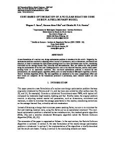
Fig. 6. NARX structure designed for reactor core identification.

distribution in the core, needs solving a large number of equations simultaneously, which, in turn, require a large amount of time and memory on digital computers. One-dimensional (1-D) and/or few point models are usually used to reduce voluminous computation, which, of course, will decrease accuracy. One way to improve accuracy and speed of the reactor core modeling, presented in this paper, is to use a neural network trained by an accurate 3-D core calculation code. Such a neural network will lead to more accurate results than 1-D or few point models. In this work, we have used DYNCO code to this purpose. DYNCO is dynamic code designed to solve Russian 3000 MWt PWR core (VVER type 320) by means of nodes distributed symmetrically in the core (Fig. 5). In VVER type 320, ten groups of control rod plus boric acid, are used to control the reactor power level and spatial power distribution in the core, while satisfying the safety criteria [21]. DYNCO can show the effects of movement of any CRGs on the core parameters, as a function of time. To do this, equations DYNCO has to solve at least near in a time step, spending a long computer time. For example, a transient of 15 h in real time, initiated by CRG movement,

needs near 1 h of computation on a Pentium II- 500 MHz computer. C. Enhancing NARX Capabilities for Identification Fig. 6 shows the NARX architecture we have used for identification of MIMO plant (VVER core) in Fig. 4. This identification model is of a series-parallel form, because during the training phase, the actual outputs of the plant (rather than that of the identification model) are fed back to the NARX inputs. The dynamic behavior of the NARX net in Fig. 6, for example output , can be described by a discrete nonlinear function of MLP inputs as

A.O

A.O (7)

are the CRGs 8, 9, 10 positions at where A.O and are the time , respectively, and Xe Xenon concentration, core thermal power, core axial offset, and

164


core reactivity at time , respectively, while represent the delay time units. The above dynamic function can be repeated for the other NARX outputs Xe, A.O, and in Fig. 6, with similar arguments and a different nonlinear function . Similar discrete nonlinear function can be driven from the four sets of core differential equations (diffusion, point kinetic, poison, and decay heat equations), using the Euler approximation of derivative terms. In this derived discrete function, and equal to the core differential equations order. Therefore, the dynamic behavior of a reactor core can be explained by a NARX net. Any CRGs movement in a PWR core, would result two effects on core dynamics: a short-term dynamic affecting the core parameters during less than 5 min, until the internal temperature feed backs overcome the input reactivity insertion and a long-term dynamics, which affects the core parameters during a time constant less than few hours, until the Xenon oscillations is stabilized in the core. But, as mentioned before, identification of systems with short and long-term dynamics is not easily and accurately possible, using a single RNN. To remove this obstacle, we tried the use of parallel NARXs, with a similar structure as shown in Fig. 7. In this structure, the first NARX is used for identification of long-term core dynamics (LNARX), the second for identification of short-term core dynamics, during any insertion of CRGs (SNARX1), and the third one for identification of short-term dynamics during any withdrawal of CRGs (SNARX2). Although identification of short-term core dynamics is also possible using one NARX, but we found that using two NARXs would result a better response during short-terms identification, specially by using separate NARXs for insertion/withdrawal of CRGs. Timing among these three NARXs, after any movement of CRGs, is regulated as follows. For the first 5 min, one of the two SNARX 1 or SNARX 2 is trained with a short time step and then, the LNARX with a long time step. The structure used for these and three NARXs is similar: 33-78-78-78-4 with (Fig. 6). In this structure, three hidden layers are composed of 78 neurons, four output units are considered for Xenon, thermal power, axial offset, and core reactivity, and 33 input units are foreseen for the present and two past delayed CRG positions, plus the present and five past delayed NARX outputs (number with and ). of inputs Although, using a smaller structure for NARXs is possible, but network responses showed that we have to use a large NARX structure, because of large number of training data and better response and prediction of network, after an on-line learning. Training algorithm in all these three NARXs is the well-known back propagation with steepest descent rule so that the total squared error (8) and the network outputs between the desired outputs at th iteration, for a data set at time is minimized over all outputs. We defined a sigmoid as (9)

Fig. 7. Multi-NARX connections for identification of long-term (LNARX) and short-term core dynamics (SNARX 1, 2).

for all neurons activation function, where is the total input of the th neuron. All NARX input data from the core, are scaled and using four following formulas: between A.O

A.O

(10) (11)

Xe

Xe

(12) (13)

where A.O is the core axial offset, is total core thermal power in Watt, Xe is average xenon concentration in (nuclei/cm ), and is core reactivity in . Two learning phases, including an off-line and an on-line learning has been used: 1) Off-Line Learning: Training a transient in RNN can be carried out by several methods e.g., instantaneous, sample period, and batch learning. — Instantaneous learning: in this method, an input and output plant data set are used at time step , and the , after the network next data set at time step , has reached below a certain value output error, [4]–[6]. — Sample period learning: a sample period of plant is used data sets, in time steps for learning until a cumulative network outputs error , has reached below during time steps, a certain value. The data set at is then omitted and will be added to the another data set at sample period. This procedure continues for the whole data sets [22]. — Batch learning: in which the entire plant data sets , during a transient, are used for learning, , has until the total transient output error, reached below a certain value, being the number of entire data sets in a transient. The main difference between the three methods lies in different selection procedure of the plant input–output data to be used for training of the neural network. While instantaneous learning uses only one set of data at each time interval, sample period learning, takes sequential data. The entire plant data sets are used in batch learning.


While instantaneous learning has been used for identification by Adali et al. [4] and Parlos et al. [5], [6], this method was deemed unsuitable for representing the network responses in our case. Reactor core is a complex nonlinear MIMO plant. The core dynamics has simultaneously two components of time and space (space distribution of power and other parameters in the core). Identification of such a system requires more powerful learning methods, compared to ordinary methods used for neural network; otherwise, the dynamic behavior of the plant cannot be adequately explored. On the other hand, the power distribution in the reactor core is a function of core history during the past few hours, mainly due to Xenon evaluation [20]. In Batch learning method the neural network is trained by the present and the history of operation of the core. The simulation results show that in this method, neural network has more ability to learn and discover the core dynamic characteristics. We used batch learning, together with the following heuristic method for calculation of the network weights, resulting in considerable improvement in responses. If the number of entire data sets in a transient is equal to , then the total transient squared error (TTSE), with scaled and values in a batch learning, will be

TTSE

(14)

The updated network weights, between th neuron in layer and th neuron in layer is (after any iteration) (15) where is the iteration number (an iteration contains all data the weight variation sets during a batch learning) and in th iteration, which can be calculated as follows: (16) is the weight difference, calculated for any where data sets at th iteration during an instantaneous learning with steepest descent rule (17) Iteration between (15)–(17) on NARX weights will reduce the TTSE in (14). The learning rate in NARXs has been selected as a variable during training iterations and among network layers. It is recalculated at any iteration, in such a manner that the average value of weights variations in any layer, be equal during the training. In our simulation, the range of its variation . This method results in uniform diswas tribution of learning pattern in all network layers and increases the network learning capability and convergence. Network training is very sensitive to initial network weights order. We selected initial network weights randomly in magni. Selecting a higher initial weights order can cause tude of saturation in neurons output and consequently no network learning, while lower initial weights order would extend the required training time. Another problem to be solved is regulating the weights during learning process, because, learning different transient

165

by network regulate the weights vector in different directions (resulting in a very large weights vector) and, hence, can cause loosing previous learning. This shortcoming could be overcome by addition of a weight difference to the network weight, defined as follows: (18) is the weight where is the number of transients and variation during each transient, computed from (16). Equations (14)–(18) must be used iteratively, until the sum of the TTSEs from all transients reaches below a certain value. The minimum number and the shape of transients required for training a dynamic plant such as nuclear reactor core, is a challenging issue. A suitable strategy should be adopted to include all possible core dynamic conditions, by movement of CRGs during the time. If we fix a period for identification i.e., 50000 s, the minimum number of transients needed for network training can be estimated. To do this, we denote CRG position by a value between 0 (fully withdrawn) and 1 (fully inserted). By dividing the period in two equal parts and assuming that CRG position during each half period can only accept 0 or 1 values, possible CRG maneuver during the period could then be represented by a binary string. Therefore, the minimum number of transients needed for network training during the whole period, using three . CRGs, would be In this work, the network off-line learning has been accomplished using 64 training transients with 50 000 s long each, until the total sum of TTSEs for all of transients, reached a value less than 1.58. The time steps for LNARX and SNARXs were selected 1800 s and 20 s respectively. Using off-line batch learning for training the network by these transients spends a long computer time. Using a decreasing trend (e.g., exponential) for expected TTSE level, will make possible for the network to be trained slowly and the weights be saved during the long training time. Fig. 8 shows the sum of ten TTSEs versus learning-iterations during off-line batch learning phase using ten transients. A learning-iteration is defined as an expected TTSE level that the network must reach for learning a transient. Expected TTSE level may be selected to decrease exponentially during the training phase as follows:

TTSE

(19)

are two adwhere Li is the learning-iteration number and justment parameters, which, in the present application, were chosen 2 and 0.5, respectively. Fig. 8 compares sum of the expected and real TTSEs. As can be seen, the network encounters an undesired increase in sum of , but after more iterations, this value will TTSE values in return to its decreasing trend. This phenomenon arises from the average network weightings in (18). Choosing an average value for any network weight may increase the TTSE in some transients and decrease it in others. The sum of TTSEs will finally decrease with more iteration. Fig. 9 shows the effects of CRGs nine and ten movements on the network, compared with the results of the DYNCO code. This test transient isn’t belong to training transients. This transient includes three short-term dynamics with each

166


behavior and enhancing reactor load following capability, fast prediction of severe operational transient and fast and accurate estimation of core safety margins. IV. INTELLIGENT NUCLEAR REACTOR CORE CONTROLLER FOR LOAD FOLLOWING OPERATIONS

Fig. 8. Sum of TTSEs for ten transients versus learning-iterations during off-line learning.

300 s long and one long-term dynamic with 68 000 s long. Therefore, the total numbers of time intervals are equaled to , where the 20 and 1800 are the time intervals of the SNARXs and LNARX, respectively. The resulting TTSE in these intervals is equal to 0.577. 2) On-Line Learning: Off-line learning is considered satisfactory when the TTSE drops below a certain value. However, further on-line learning is deemed necessary after acquisition of a new data set that capturing any process dynamics not included in the training set and tracking slow process parameter drifts. The weights are then updated through acquisition of new data set. For on-line learning, (14)–(17) are used again during a batch learning until a certain time . This online learning is useful when data acquisition from a real plant is used for accurate prediction of the plant behavior. Fig. 9 shows the effect of the same inputs on the network, when the network training is improved by on-line learning until 30 000 s, with a TTSE less than 0.01. As can be seen in Fig. 9, the network prediction after 30 000 s are nearly matched with the plant data during further steps. D. Advantages and Applications Complete structure shown in Fig. 7, is able to simulate a transient of 50 000 s real time, in less than 5 s, with an average TTSE per time step lees than 0.01, on a Pentium II 500 MHz (using the C++ language). Same transient would require about 50 min computation time using DYNCO code. Therefore, the NARX is about 600 times faster with an acceptable average TTSE error. Accessing to all dynamics state variables at the network input is possible, by NARX special structure in Fig. 6. Therefore, beginning from desired initial core conditions, just needs implementing the present and five past saved core states, plus present and two past saved CRGs positions to the NARX inputs. In RLMP structure used by Parlos et al. for identification of a steam generator [5], [6], the network neurons included “hidden states.” Therefore it was not possible to start with desired plant initial conditions. Such structure is always limited to be started from constant initial conditions. This identification method can extensively be used in nuclear reactor control such as fast prediction of the reactor dynamic

Load following operations in nuclear power plants encounter difficulties, compared to with fossil fuel power plants. These difficulties mainly arise from nuclear reactor core limitations in local power peaking, while the core is subject to large and sharp variation of local power density during transients. Nuclear reactor core is a complex nonlinear MIMO plant, in which the variables are strongly coupled, therefore, CRGs maneuvers, can induce unintended time-space Xenon oscillations, resulting in large local power peaking. Local power peaking is also a function of the reactor power level and fuel burn up. In a manual core control system during load following operation, the operator chooses the best CRGs maneuver in any time interval, based on his knowledge and experience. Many automatic control systems have been developed to improve the plant load following capabilities during last three decades. In recent years, increasing speed of digital computers, together with design of advanced neural networks and fuzzy systems, enabled engineers to design simple, and on-line intelligent control systems for nuclear plants (core, steam generator ). Based on the available references [23], the load following is not normally done in VVER reactors and the plants are designed basically for base-load operation. However, these plants are planning to develop and implement a new automated core power distribution control system that will operate under supervision of the operators. In western plants, even when the plant is basically base-loaded, it is a common practice to still evaluate the impact of load following operations, as far as overall safety impact is considered. The core control system design of VVER is in general similar to western practices. However, there are some differences on core control strategies. The core control strategy of VVER is mainly based on the manual control of power peaking, with the requirement to keep them within prescribed limits using in-core instrumentation. The power distribution is allowed to change continuously which results in some Xenon oscillations. Axial oscillations in VVER reactor are nondivergent. However, in the case of their occurrence, the values of the core thermal parameters can increase. A. Axial Off-Set Control During Load Following Operation A nuclear power reactor core controller has to control the core thermal power along with the safety limitation on local power peaking during load following operation. Local power peaking in nuclear reactors, is a complex 3-D phenomenon, resulting from different reactor parameters (fuel loading, power level, temperature distribution, position of CRGs, fuel burn up, spatial Xenon oscillations ). To simplify this phenomenon, local power peaking is usually divided into two radial and axial components. While radial power peaking is usually flattened (via an optimal fuel loading/reloading pattern) once at the beginning of cycle (BOC), the axial power peaking is continuously changing


167

Fig. 9. Effects of movement of the control rods groups (CRGs) nine and ten on core parameters comparing with multi-NARX outputs without on-line learning and with on-line learning between 0–30 000 s. (a) CRGs movement. (b)–(e) DYNCO code and multi-NARX responses.

by perturbations created by CRG maneuvers. A.O is the parameter usually used to determine the core power peaking. This parameter, which could be easily measured on-line, via ex-score instrumentation, still reduces the complexity of the problem and provides an efficient practical mean to control the reactor. Thus, the main challenge of the reactor control, during load following operation, is to maintain the axial power peaking (represented by A.O) within certain limits, about a reference target value.

The limitations on the core A.O can be analyzed in coordinates. Where is the normalized A.O defined by A.O

(20)

is relative core thermal power (the ratio of the actual where core thermal power to nominal thermal power).

168

Fig. 10.


Intelligent core controller structure.

In constant axial offset strategy (C.A.O), the limitations on the core A.O value can be shown by two parallel lines in coordinate [20]. This means that the core working conditions in coordinates must lie within a certain band (i.e., %) during any power transient. The target A.O chosen is that would occur at full power, equilibrium Xenon, and all rods out. This control strategy protects the reactor from any divergent Xenon oscillation and would ensure safe operation of the reactor during load following transients. Finally, it worth to point out that, in such a C.A.O control strategy, the use of a fuzzy critic in an intelligent core controller is more suited to this type of problem, because we have to main) within predetertain the reactor working condition bands), rather than to control the exact axial mined limits ( power peaking, employing crisp logic.

B. The Intelligent Nuclear Reactor Core Controller In this research, we used DYNCO code, as the real plant, for testing and tuning of the designed controller. 1) Controller Structure: Fig. 10 shows the structure of the designed intelligent core controller. The control algorithm used includes the following steps. Step 1) Defining: the expected core thermal power ; the maximum and minimum overlapping between O.L and the maximum the CRGs O.L and minimum of allowable core axial offsets A.O A.O during the next time interval. This step is performed by the Modules 1 and 2, which constitute the inputs of the controller.


Step 2) Generating all possible CRGs maneuvers (h8, h9 and h10 indicate the positions of the CRGs number eight, nine, and ten, respectively), taking into account the initial CRGs positions, and the maximum and minimum overlapping between the CRGs. This is performed by the Module 3. Step 3) Implementing each of CRGs maneuvers to the trained NARX core model and predicting the core response during the next time interval (Module 4). Step 4) Finding optimum response of the core model and the related CRGs maneuver (Modules 5, 6, and 7). Step 5) Implementing the best CRGs maneuver to the DYNCO code, as the real plant (Module 8). Step 6) Updating the NARX core model, using the response of the real plant (DYNCO code). The above steps are executed at each time interval during the transient. Detailed descriptions of the different modules are explained below. 2) CRGs Maneuver Generator: Module 3 is used as a CRGs maneuver generator. Possible CRGs maneuvers can be generated during each time interval, given the length and speed of the CRGs; their initial positions and overlapping between the CRGs are known. The length and speed of the CRGs in VVER type 320 are 350 cm, and 2 cm/s, respectively. The maneuvers generator in Module 3 generates 60 maneuvers for each overlapping value and O.L . Each of these 60 maneuvers may between O.L generate a different transient in the reactor core. 3) The NARX Core Model: A VVER type 320 reactor core at the BOC, as was mentioned in Section III-A and Fig. 4, has been used again as reference plant. The VVER type 320 has been designed for base load operation. Load following capability has not been considered in designing of the CRGs. To study the reactor load following capabilities, we had to decrease the reactivity of CRGs number eight, nine, and ten, by the coefficients of 0.5, 0.4, and 0.3, respectively (using these as gray rods). Module 4 in Fig. 10 includes the neural network core model used for identification of the plant. This model includes a single NARX, which is used for identification of long-term core dynamics with a time interval equal to 300 s. This NARX core model had been already trained by an off-line batch learning, using 64 transients simulated by the DYNCO code. These transients include all possible core dynamic conditions, by movement of CRGs during a fixed period of 10 000 s. We have not used boric acid as a control agent, to avoid sharp increase in number of required transients and the training time. 4) Analyzing the Predictions of the Core Model: Each of CRGs maneuvers generated in Module 3, causes a different transient in the reactor core (variation of the A.O and power). We need a suitable method to analyze the predicted plant response with regard to the core A.O limitation and to find the optimum CRG maneuver. We defined two parameters PIR and PIL, to compare the predicted core model responses with A.O limitation (Fig. 11) PIR

(21)

169

1( ( [ ( + 1)])

)

Fig. 11. Minimum and maximum limitations on core I I ; I and the predicted core I I , between the relative core thermal power values at the mth P t m and the next time intervals P t m .

1( ( [ ( )])

)

( ) and the expected ( ) core relative thermal ( ( )) and the next time intervals ( ( + 1)).

Fig. 12. Predicted P powers, at the mth t m

P

t m

PIL

(22) and are the th and the next time intervals, is the relative core thermal values at the th and are the time interval, at the maximum and minimum limitations of the core th time intervals, I is the predicted core for a CRGs are positive constant coefficients that are maneuver and used for scaling the parameters. Each of these two parameters can be positive, zero, or negative. If PIR and PIL were both positive, then the predicted core working condition would be within the A.O limitation band. If one were positive and the other negative, the predicted core working condition would be out of the allowable A.O limitation band (Fig. 11). We defined another parameter (power error) between the predicted and the expected core power (Fig. 12) as where

PT

(23)

and are the predicted where th and the expected relative core thermal powers at the time interval and is a positive constant coefficient that is used for scaling the parameter. This parameter can be positive, zero, or negative. If PT were zero, the predicted core thermal power would be matched with the expected one, during the next time interval.

170


TABLE I 27 FUZZY CRITIC RULES

Fig. 13.

(a) Output Gaussian membership functions of the fuzzy critic. (b)–(d) Inputs Gaussian membership functions of the fuzzy critic.

Module 5 calculates three parameters of PIR, PIL and PT for each of the transients predicted by the NARX core model. 5) Fuzzy Critic: The Module 6 is a fuzzy system designed for analyzing each of the transient generated by CRG maneuver. This module examines any core model response with regard to the core A.O limitations and the power error. This fuzzy system contains a singleton fuzzifier, a product inference engine, and a center of gravity defuzzifier (SF-PIE-CGD). Inputs of the fuzzy system include PIR, PIL, and PT parameters, and output of defuzzifier is a crisp value that shows the suitability degree of the input parameters (core model responses). The most important part of this fuzzy system is the fuzzy rule-base, which should be written by an expert (the operator) using his knowledge and experience for decision-making at any core states, during load following operations. Table I includes 27 rules defined to this

purpose. The inputs of the fuzzy rule-base, shown in Fig. 13 are Gaussian membership as follows: if (24) if (25) if (26) if where is one of the three parameters: PIR, PIL and PT. The membership functions of the output are also Gaussian membership functions as (27)


Fig. 14. Core controller results for a 16-2-4-2 load following using local on-line learning. (a) Expected and real core thermal powers. (b) Core and real core I . (c) Control rod groups (CRGs) number 8, 9, 10 positions. (d) CRGs over lapping value.

1

where is equal to . The 27 rules in Table I cover all different possible state with three inputs PIR, PIL, and PT. The Gaussian membership functions in (27) will imply the . The last three crisp output value of vary between rules in Table I will never be initiated in a transient, therefore, . the crisp output will varies between 6) Optimum CRGs Maneuver Finder: The output from the fuzzy critic (Module 6), represents the suitability degree of the core model responses. The optimum CRG maneuver corresponds to the largest -value. Therefore, the Module 7 must be a maximum -value finder. The Module 7 will implement the optimum maneuver found, to the real plant (DYNCO code). This optimum determines the optimum overlapping value and the positions of the three CRGs, for the next time interval. 7) Updating the NARX Core Model: After the optimum CRG maneuver is implemented to the DYNCO code (as the real plant), the responses will be used for updating the NARX core model, using on-line batch learning. On-line learning is necessary after acquisition of a new data set for capturing any process dynamics, which was not included in the training set. The starting point of this batch learning is fixed at the beginning of the load following transient. On-line batch learning may be accomplished using the initial off-line batch learning weights matrix “global on-line learning” or the results of the on-line

171

1I limitations

batch learning weights matrix at the previous time interval “local on-line learning.” Each of these two methods represents advantages and deficiencies in intelligent core control (see Section IV-C). C. Implementation and Results In this project, we used the C++ language to build the intelligent core controller (Fig. 10) and the DYNCO code to represent the real plant. Selection of the time interval for controlling the core during a transient depends on the: execution time of the control algorithm and maximum rate of power change during load following. In the following simulations, a time interval of 300 s was selected. and in (21)–(23) were selected as 10, The constants 10, and 5, respectively. To evaluate validity of the results of the core controller, during different load followings, we defined an average power error (APE) parameter as

APE

(28)

is the total number of time intervals, and are the real and the expected core thermal powers at the th time interval, respectively.

where

172


Fig. 15. Core controller results for a 16-8 load following using local on-line learning. (a) Expected and real core thermal powers. (b) Core real core I . (c) Control rod groups (CRGs) number 8, 9, 10 positions. (d) CRGs overlapping value.

1

1) Local On-Line Learning: Figs. 14, 15 show the results of the designed intelligent core controller with local on line learning in two different cases. The overlap between CRGs number 8, 9, 10 has been limited between 0% to 40%, and the limited to % %( % corresponds allowable core to the A.O at nominal power) Case 1: The first load following considered was a 16-2-4-2 transient shown in Fig. 14. This transient includes a slow decrease of the core power from 100% to 50% during 2 h, constant power at 50% for 4 h, and slow return to full power during 2 h. The total transient time was 35 800 s divided in 119 time intervals. This case resulted in an APE equal to 53.6 MWt (less than 1.8% of nominal power). Case 2: The second load following considered was a 16-8 transient shown in Fig. 15. This transient includes a fast decrease of the core power from 100% to 70% with a rate of 2%/min, constant power at 70% for 8 h, and fast return to full power with a rate of 5%/min. The total transient time was 34 600 s, divided time intervals. This case resulted in an in APE equal to 40.6 MWt (less than 1.4% of nominal power). The total execution time of the designed intelligent core controller on a Pentium IV 1.4 MHz PC falls to less than 150 s, from which 40 s is spent for local on-line learning and the remaining 110 s for other algorithm steps. Computation time may be considerably reduced by using parallel processing of the control algorithm, and/or faster computers.

1I limitations and

2) Global On-Line Learning: Figs. 16, 17 show the results of the designed intelligent core controller with global on line learning in the same above cases. Case 1: Fig. 16 compares, the results of the intelligent core controller for a 16-2-4-2 transient as in Fig. 14, using global and local on-line learning. This case resulted in an APE equal to 43.3 MWt (less than 1.5% of nominal power), using global on-line learning. Therefore the APE is decreased by 0.3% of nominal power. Case 2: Fig. 17 compares, the result of intelligent core controller for a 16-8 transient as in Fig. 15, using global and local on-line learning. This case resulted in an APE equal to 28.1 MWt (less than 1% of nominal power), using global on-line learning. Therefore the APE is decreased by 0.4% of nominal power. The APE values prove that using global versus local on-line batch learning, improves the intelligent controller results. Global on-line batch learning, using the whole plant data since the beginning of the transient, regulates the network weights in any time interval. Therefore, as the transient time extends, the computer execution time may increase between few minutes to few hours. In this research, we have not used boric acid as a control agent. Boric acid has an important role in controlling the power level and A.O at the end part of the long transients. This deficiency can be seen, when the CRGs reach to the top of the core


Fig. 16. Comparing core controller results for a 16-2-4-2 load following using local and global on-line learning. (a) Core power. (b) Core core I .

1

Fig. 17. Comparing core controller results for a 16-8 load following using local and global on-line learning. (a) Core power. (b) Core core I .

1

in Figs. 16 and 17, after 28 700 s and 32 000 s, respectively. The use of boric acid may still reduce the APE. V. DISCUSSION Generally, identification can be implemented via provision of input–output data sets as a lookup table. However, this will lack the required flexibility considering uncertainties that are involved. A suitable alternative for identification of systems with complex dynamics is to utilize flexible identification tools where identification with minimal error, does not lose validity even in the presence of uncertainties and maximal generalization capability, rather than just data fitting. Among such tools, artificial intelligent systems and especially ANNs and fuzzy systems can be mentioned. ANNs are powerful and flexible tools for carrying out realworld complex tasks. An ANN can function as a content-addressable memory where data is stored and retrieved in a distributed manner [13]. The function of a content addressable memory is to retrieve a pattern (item) in response to the presentation of incomplete or noisy prototypes. The ANN gives pos-

173

1I limitations and real

1I limitations and real

sible good guesses about missing information, even though we may lack accurate data or perhaps all data in certain ranges. It is clear that the achievement of any identification method depends on ability to represent a suitable model in real conditions. This in identification context is called persistency of excitation. It means that the system must be excited with rich enough inputs, where all of the dynamic abilities of the considered system are made apparent. The use of 64 transient, mentioned in Section III-C1 and the average network weights in (18), have been used for this purpose. Therefore, this method includes rich enough training data sets. It is worth noting that any robust identification method is valid only in a certain range of inputs–outputs and uncertainties, not for all regions of disturbances and/or uncertainties. Using neural network method in this context despite its dynamic flexibilities is no exception. The extent of these uncertainties/disturbances can be evaluated via analytical methods; however, flexible methods may be adopted even if there are no specific or analytical bounds for disturbances and/or uncertainties. On the , other hand, in contrast to purely analytical techniques like for which validity is guaranteed only for a limited class of un-

174


certainties/disturbances, flexible methods may maintain reasonable validity for a wider range of disturbances and uncertainties. Having considered all the benefits versus the limitation of artificial intelligence approaches, one may evaluate the performance of the approach by introducing a set of all possible disturbances/uncertainties and then observing the results after change of, e.g., amplitude of disturbance. This research work aims to contribute to the development of new methods to tackle one of the most complicated problems of modern PWRs, i.e., improvement of load following capability of the plant, using advanced intelligent controllers. It is obvious that further steps, i.e., uncertainty analysis, stability analysis, use on a full scope simulator, and etc., are still to be undertaken toward practical application in nuclear power plant. One of the potential applications of this method may be in the design and development of computerized operator decision aids (CODA) or support system (COSS). Furthermore, the following points are to be considered in practical application of the proposed method: The RNN can be trained by data recorded from the plant load following operations during a sufficient time period; the control algorithm may be executed by parallel processing or by a very fast computer and the boric acid should be added as a core control agent.

VI. CONCLUSION Discovering long-term dependencies with gradient descent in the identification of dynamic plants has been a complex not circumvented by recurrent neural networks. In this paper, a multi-NARX structure for identification of a complex nonlinear plant was used and a training method for learning short- and long-term dynamics was developed. The potential of RNNs in modeling complex nonlinear plants and fast prediction of core dynamic behavior can be used in designing an intelligent reactor core controller. This paper proposes a control system for optimal CRG maneuvering and overlapping during load following operations. Unlike previous approaches, where simplified SISO models are used for training and testing is performed on complex nonlinear MIMO data, the proposed approach employs DYNCO code complex nonlinear MIMO data both for training and testing. This controller can be used with variable control rod overlapping strategy, which, in turn, increases the core capabilities for load following operations. On the other hand, the fuzzy critic laws, used in this intelligent controller, can be modified by expert (the operator), thus improving the results. Using global versus local on-line batch learning, for updating the NARX core model, improves the responses in terms of error reduction. However, it increases the algorithm execution time. This difficulty can be removed using faster computers and/or parallel processing. The proposed methodology represents an innovative method for identification and control of complex nonlinear plants and may improve the responses compared to other control approaches.

ACKNOWLEDGMENT The authors would like to thank the anonymous reviewers for their helpful comments, which improved the content of the paper. REFERENCES [1] H. L. Akin and V. Altin, “Rule-based fuzzy logic controller for a PWR-type nuclear power plant,” IEEE Trans. Nucl. Sci., vol. 38, pp. 883–890, Apr. 1991. [2] C. C. Kuan, C. Lin, and C. C. Hsu, “Fuzzy logic control of steam generator water level in pressurized water reactors,” Nucl. Technol., vol. 100, pp. 125–134, Oct. 1992. [3] M. G. Na and B. R. Upadhyaya, “A neuro-fuzzy controller for axial power distribution in nuclear reactors,” IEEE Trans. Nucl. Sci., vol. 45, no. 1, pp. 59–67, Feb. 1998. [4] T. Adali, B. Bakal, M. K. Sonmez, R. Fakory, and C. O. Tsaoi, “Modeling core neutronics by recurrent neural networks,” in Proc. World Congress on Neural Networks, vol. 2, Washington, DC, June 1995, pp. 504–508. [5] A. G. Parlos, A. F. Atiya, and K. T. Chong, “Nonlinear identification of process dynamics using neural networks,” Nucl. Technol., vol. 97, pp. 79–96, Jan. 1992. [6] A. G. Parlos, K. T. Chong, and A. F. Atiya, “Application of the recurrent multi-layer perceptron in modeling complex process dynamics,” IEEE Trans. Neural Networks, vol. 5, pp. 255–266, Mar. 1994. [7] K. S. Narendra and K. Parthasarathy, “Identification and control of dynamical systems using neural networks,” IEEE Trans. Neural Networks, vol. 1, pp. 4–27, Mar. 1990. [8] T. Lin, B. G. Horne, P. Tino, and C. L. Giles, “Learning long-term dependencies in NARX recurrent neural networks,” IEEE Trans. Neural Networks, vol. 7, pp. 1329–1338, Nov. 1996. [9] M. S. Roh, S. W. Cheon, and S. H. Chang, “Thermal power prediction of nuclear power plant using neural network and parity space model,” IEEE Trans. Nucl. Sci., vol. 38, pp. 866–869, Apr. 1991. , “Power prediction in nuclear power plants using a back-propaga[10] tion learning neural network,” Nucl. Technol., vol. 94, pp. 270–278, May 1991. [11] M. Boroushaki, M. B. Ghofrani, and C. Lucas, “Identification of a nuclear reactor core (VVER) using recurrent neural networks,” Ann. Nucl. Energy, vol. 29, no. 10, pp. 1225–1240, July 2002. [12] M. Boroushaki, M. B. Ghofrani, C. Lucas, and M. J. Yazdanpanah, “An intelligent nuclear reactor core controller for load following operations, using recurrent neural networks and fuzzy systems,” Ann. Nucl. Energy., vol. 30, no. 1, pp. 63–80, Jan. 2003. [13] S. Haykin, “Dynamically driven recurrent networks,” in Neural Networks a Comprehensive Foundation. Englewood Cliffs, NJ: PrenticeHall, 1999, ch. 15, pp. 732–783. [14] L. X. Wang, “Part II: Fuzzy system and their properties,” in A Course in Fuzzy Systems and Control. Englewood Cliffs, NJ: Prentice-Hall, 1997, pp. 90–117. [15] L. R. Medsker and L. C. Jain, “Learning long-term dependencies in NARX recurrent neural networks,” in Recurrent Neural Networks Design and Applications. Boca Raton, FL: CRC Press, 1999, ch. 6, pp. 133–146. [16] Y. Bengio, P. Simard, and P. Frasconi, “Learning long-term dependencies with gradient descent is difficult,” IEEE Trans. Neural Networks, vol. 5, pp. 157–166, Mar. 1994. [17] L. J. Hamilton and J. J. Duderstadt, “The calculation of core power distribution,” in Nuclear Reactor Analysis. New York: Wiley, 1976, ch. 13, pp. 111–117; 525–529. [18] K. Ogata, “Z transform,” in Discrete Time Control Systems. Englewood Cliffs, NJ: Prentice-Hall, 1987, ch. 2. [19] T. W. Kerlin, G. C. Zwingelstein, and B. R. Upadhyaya, “Identification of nuclear systems,” Nucl. Technol., vol. 36, pp. 7–37, Nov. 1977. [20] P. J. Sipush, A. P. Ginsberg, and T. Morita, “Load following demonstrations employing constant axial offset power distribution control procedures,” Nucl. Technol., vol. 31, pp. 12–31, Oct. 1976. [21] F. Yousefpour and I. P. Balakine, Yadernaya Energetica, no. 6, 8, 1997. [22] S. Omatu, M. Khalid, and R. Yousof, “Neuro-control techniques,” in Neuro-Control and Its Applications. London, U.K.: Springer-Verlag, 1996, ch. 4, pp. 116–121. [23] Core Control and Protection Strategy of VVER-1000 Reactors, Apr. 18–22, 1994.