Statistitcal Methods & Applications (2001) 10:49~55
SMA
@ Springer-Verlag 2001
Identification of vector AR models with recursive structural errors using conditional independence graphs Marco Reale 1, Granville Tunnicliffe Wilson 2 1 Mathematics and Statistics Department, University of Canterbury, Private Bag 4800, Christchurch, New Zealand (e-mail:
[email protected]) 2 Mathematics and StafisticsDepartment, Lancaster University, LancasterLAl 4YE United Kingdom (e-mail: g.tunnicliffe-wilson @lancaster.ac.uk)
Abstract. In canonical vector time series autoregressions, which permit dependence only on past values, the errors generally show contemporaneous correlation. By contrast structural vector autoregressions allow contemporaneous series dependence and assume errors with no contemporaneous correlation. Such models having a recursive structure can be described by a directed acyclic graph. We show, with the use of a real example, how the identification of these models may be assisted by examination of the conditional independence graph of contemporaneous and lagged variables. In this example we identify the causal dependence of monthly Italian bank loan interest rates on government bond and repurchase agreement rates. When the number of series is larger, the structural modelling of the canonical errors alone is a useful initial step, and we first present such an example to demonstrate the general approach to identifying a directed graphical model. Key words: Partial correlation, moralization, causality, graphical modelling, lending channel
1 Introduction The canonical pth order vector autoregressive model, VAR(p), of a stationary, m dimensional time series x t = (xt,1, x t , 2 , . . . , x t , ~ ) ' is of the form: X t = C -}- ~ l X t _
1 + ~2Xt_2
+ 9 . . q- q ~ p X t _ p -]- e t
(1)
where c allows for a non-zero mean of x t and et is multivariate white noise with general covariance matrix V. Our working assumption is that the series is Gaussian but our methods should be applicable under wider conditions, such as et being I.I.D., presented for example in Anderson [2]. This model is attractive because
50
M. Reale, G. Tunnicliffe Wilson
its estimation from a sample Zl, x 2 , . . . , Xn, by least squares applied separately to each component of x t , is straightforward. For large sample length n it is also fully efficient provided there are no subset constraints on these separate regressions, (Judge et a l [ 11]), the properties of the estimates given by the regression are reliable, and the estimate of V is independent of the estimates of ~k. The order p of the regression may be determined by various methods including inspection of a multivariate partial autocorrelation sequence, see Reinsel [16], pp 69-70, or minimization of an order selection criterion such as AIC, Akaike [1], HIC, Hannan and Quinn [9], or SIC, Schwarz [17]. Such criteria have been extensively used in time series contexts. Recently Swanson and White [20] have used them for linear and non-linear modeling of multiple time series and in our examples we also tabulate their values as an aid to model selection. There are various approaches to multiple time series modeling which seek either to transform models such as (1) to a form which includes contemporaneous relationships among the variables, or to identify directly such a form, see for example Box and Tiao [6] and Tiao and Tsay [21]. Our aim in this paper is similar; our approach is to consider the structural autoregressive model of the same form as (1) but with the addition of contemporaneous dependence through a matrix coefficient ~o: ~oxt = d + ~Xt-1
Jr- ~ X t - - 2
~- " " " -~- ~ ; X t - - p
q- a t .
(2)
The general relationship between time series and structural econometric models was developed by Zellner and Palm [24]. In our present context the equivalence between (1) and (2) is given by ~ = ~0~i and ~ o e t = at. A requirement of (2) is that the variance matrix D of at is diagonal. We require a further condition on ~0, that it represents a recursive (causal) dependence of each component of x t on other contemporaneous components. This is equivalent to the existence of a re-ordering of the elements of x t such that ~0 is triangular with unit diagonal. Each possible ordering of x t therefore gives a potentially distinct form of (2), but these are all statistically equivalent, corresponding to factorizations of V - 1 =- ~ b ~ D - l ~ 0
.
(3)
This contrasts with the unique form of (1), which is the attractive feature of that model from a time-series modeling viewpoint. The value of (2) therefore lies in the possibility that there is one particular form which, as a consequence of its representing a true simple mechanism, is more parsimonious in its parameterization than either (1) or the other forms of (2). This would be reflected in the ability to exclude many of the elements of ~o and ~* from the model without penalizing the fit in comparison with the saturated forms of either (1) or (2). Identification of such a model may then provide added insight into the true mechanisms which generate the data. That is what we seek to achieve by the method described in this paper. However we introduce this method in section 2 without reference to dynamic structure. The relationship (3) shows that some, though not necessarily complete, information on the structure of ~b0 is available from the variance matrix of the innovations. We
VAR identificationusing conditional independence graphs
51
therefore first illustrate the method, in section 2, without reference to any lagged structure, by its application to an innovation series et. This arises from a canonical autoregressive-moving average (ARMA) model fitted to a series of seven daily dollar term interest rates. In section 3 we consider how the method may then be extended to identify structural autoregressions. Section 4 contains an example which illustrates this approach using three monthly monetary time series.
2 Recursive structure and partial correlations Neglecting, for the present treatment, any effects of time series model estimation, we suppose that we have observations on the vector Gaussian white noise innovations process et with the usual sample covariance matrix ~r. We wish to determine from the data the form of possible sparse structural matrices #0 which are compatible with V. There may be no unique such form without imposing further constraint using insight from the modeling context. Swanson and Granger [19] consider an almost identical problem, but focus more on testing for the constraints which are implied by a particular structural form of #0 which has commonly occurred in practice. Their tests are expressed in terms of partial autocorrelations which, as they remark, are not directional and would therefore appear less appropriate for recursive (causal) models. We also use pair-wise partial autocorrelations, but conditioning on all remaining variables (i.e. components of et) rather just one other variable at a time. This is because such partial correlations are used to construct the conditional independence graph (CIG) of the variables, following procedures presented for example in Whittaker [23]. As Swanson and Granger also remark, the structural form of dependence between the variables is naturally expressed by (and is equivalent to) a directed acyclic graph (DAG), in which nodes representing variables are linked with arrows indicating the direction of any causal dependence. A DAG implies a single CIG for the variables, but the possible DAGs which might explain a particular CIG may be several or none. The point is that, subject to sampling variability, the CIG is a constructible quantity and a useful one for expressing the data determined constraints on permissible DAG interpretations. The CIG consists of nodes representing the variables, two nodes being without a link if and only if they are independent conditional upon all the remaining variables. In a Gaussian context this conditional independence is indicated by a zero partial autocorrelation:
p (et#, et,y]{et,k, k # i, j}) = O.
(4)
In the wider linear least squares context, defining linear partial autocorrelations as the same function of linear unconditional correlations as in the Gaussian context, (4) still usefully indicates lack of linear predictability of one variable by the other given the inclusion of all remaining variables. The link with Granger causality is quite evident. The set of all such partial correlations required to construct the CIG is conveniently calculated as p (et,i, et,y I{e~,k, k # i, j}) = -Wiy/x/~(WiiWjj)
(5)
52
M. Reale, G. Tunnicliffe Wilson
US Dolor 6 month, 2 year and 10 year term interest rotes 11.010.5 10.0 -
,W,
,."
9.5-
~,~.
~0,
a
,
.
,',
9.0. ,
8.5. c-
' .~;,,
: 8 , ~ ,~I, .,~ ~
,"d"" , 8.0 -J
L.,.;
7.5 ! 7.0
Days from ,30 November 1987 Fig, 1. Six-month (solid line), two year (broken line) and ten year (dotted line) dollar term rate series
where W = V -1. The sample values are obtained by substituting the sample value
f~ofV. Our example uses the innovations from the series of daily dollar term rates over the period from 30th November 1987 to 12th April 1990, excluding non-trading days. The maturity terms are 6 month, 1, 2, 3, 5, 7 and 10 years. Fig. 1 illustrates just the six month, two year and ten year rates. The movements in the series are clearly highly correlated as supported by Table i which shows the correlation matrix of the linear innovations from a well-fitting canonical ARMA(1,1) model estimated for these seven series. These residual are related only by this contemporaneous correlation. Plots of their auto- and cross-correlations from lags 1 to 20 showed no evidence of departure from multivariate white noise, with almost all values within the two standard error limits (0.082) of zero. The multivariate portmanteau test statistic of Hosking [10], for multivariate white noise, was 961.3 on 882 degrees of freedom. This is close to the upper 2 89percentage point, but for a series of length 600 it indicates a very good fit. The distribution of some of the residual series showed evidence of long tails, as is usual for such financial indicators. The sample kurtosis varied from 1.3 to 12.9, but the skewness was generally small. All our procedures are based on time series sample correlations whose asymptotic distribution, see Priestley ([14], p. 339), is unaffected by non-zero (but finite) kurtosis, so that tests based upon Gaussian assumptions remain valid in large samples. Table 2 shows the corresponding matrix of partial autocorrelations as defined by (5).
VAR identification using conditional independence graphs
53
Table 1. Correlation coefficients of dollar term rate innovations
et,1 et,2 et,3 et,4 et,5 et,6 et,7
1.000 0.799 0.516 0.502 0.452 0.418 0.420
1.000 0.538 0.515 0.458 0.425 0.423
1.000 0.944 0.883 0.838 0.812
1.000 0.924 0.887 0.863
1.000 0.965 0.941
1.000 0.967
et,1
et,2
et,3
et,4
et,5
et,6
1.000 et,7
Table 2. Partial correlation coefficients of dollar term rate innovations with * indicating significance at the 5% level
et,1 et,2 et,3 et,4 et,5 et,6 et,7
1.00 *0.720 0.022 0.037 0.019 --0.045 0.038
1.00 *0.113 0.017 --0.021 --0.012 0.006
1.00 *0.689 "0.154 --0.050 --0.055
1.00 *0.270 0.042 0.010
1.00 *0.543 "0.115
1.00 *0.658
1.00
et,1
et,2
et,3
et,4
et,5
et,6
et,7
Some of these are marked to show significance at the 5% level. The significance levels are obtained by using the relationship between a regression t value and the sample partial correlation/5 given by/5 = t/v/((t 2 + u) (see Greene [8], p. 180). Here v is the residual degrees of freedom in the regression of one of the variables in the partial autocorrelation, upon all the other variables. The t value is that attached, in this regression, to the other variable in the partial autocorrelation. This is a relationship deriving from the linear algebra of least squares, and is not reliant upon statistical assumptions. Standard assumptions are needed to support the usual distribution of t under the null hypothesis that the true value of the relevant variable is zero, which is equivalent to p = 0. There are of course statistical pitfalls in applying the test simultaneously to all sample partial autocorrelations. Our attitude is similar to that advocated by Box and Jenkins [5] for the identification, for example, of autoregressive models using time series partial autocorrelations. We use these values to suggest possible models; after fitting these we apply more formal tests and diagnostic checks to converge on an acceptable model. In this example the critical value for significance at the 5% level is an absolute partial correlation exceeding 0.081. In fact all the marked values exceed the 1% critical value of 0.106, but we indicate the three lower valued significant partial correlations with broken lines in Fig. 2 which represents the tentative conclusions from Table 2 as a CIG. It's form is almost that of the linear structure which was investigated by Swanson and Granger. This figure was presented and discussed by Tunnicliffe Wilson [22] but without any further modeling. Central to the interpretation of a CIG is the separation theorem. The CIG is constructed by pairwise separation of variables which are independent conditional on the remainder. The separation theorem states that if two blocks of variables are separated, i.e. there is
54
M. Reale, G. TunnicliffeWilson
/
9169
", /
....... 9 1 6 9 1 6 9 1 6 9
Fig. 2. ConditionalIndependenceGraphderivedfromTable2 for the dollar termrate innovationseries no link between any member of the first block and any member of the second, then the two blocks are completely independent conditional on the remaining variables. See for example Whittaker ([23], pp. 64-67) for a general proof and references to more straightforward proofs in the Gaussian case, where the result can be read directly from the joint density. To illustrate the theorem, Fig. 2 implies that { 1,2} are independent of {6,7} given {3,4,5 }. Using a straightforward notation for joint and conditional densities, the first part of (6) is a consequence of this CIG. Similar arguments lead to the remaining parts of (6). fl...7 = fl,213,4,5f3,4,5f6,713,4,5 = fl,213f3,4,5f6,715 = fa12f213f3,4,5f6,TIr"
(6)
This brings us to the next step which is to determine what DAG structures can explain this CIG, and to estimate them. This is part of a much wider problem of the search for causal structure, covered for example by Spirtes, Glymour and Scheines [18]. The procedure to determine the CIG implied by a given DAG has become known as moralization, following Lauritzen and Spiegelhalter [13]. A node B in a DAG is a parent of a node A if there is an arrow f r o m B directly linking to A. Moralization is the construction of a CIG by linking (marrying), for each node of a DAG, all of its parents. The original links are retained with their directional arrows deleted. In the Gaussian context it can be seen from (3) that moralization corresponds to the creation of non-zero entries in V - I , which characterizes the CIG, from the non-zero entries in ~0, which characterizes the DAG. If the graph in Fig. 2 were linear, with no links et,3 - et,5 or et,5 et,7, there would be just seven possible DAG interpretations. These are obtained by choosing one node as a root o r p i v o t and directing all arrows away from it. Arrows could not come together as that would create a new, moral, link. The links et,3 et,5 and et,5 - et,z introduce more possibilities. These can be listed by first considering the possible DAG interpretations of sub-graphs of Fig. 2 as shown in Table 3. Selected sub-graphs, one from each column, can be re-assembled to construct an overall DAG. This can only be done however, without creating a new moral link, provided neither nodes 3 or 5 have parents in two components. This results in 28 possible combinations: -
-
-
1)c~Aa; 8)/3Cc; 15)~,Da; 22)-/Eb;
2)aAc; 9)TAa; 16)'yDb; 23)'7Ec;
3)aCa; 10)TAc; 17)~,Dc; 24)3,Ed;
4)c~Cc; 1 l)~/Ba; 18)'~Dd; 25)-yEe;
5)/3Aa; 12)7Bc; 19)q,De; 26)-yEf;
6)/3Ac; 13)7Ca; 20)TDf; 27)7Fa;
-
7)/3Ca; 14)~/Cc; 21)flEa; 28),'/Fc.
All these models are in fact statistically equivalent, as factorizations such as 6 readily confirm. They may be estimated with full efficiency by separate regressions. For example Fig. 3 shows one possible DAG, 7Aa, with values attached to the links
VAR identification using conditional independence graphs
55
Table 3. Possibledirected subgraphs
Q
(Y
9
(3
@
O
o,0 _ _ _ . 0 .........(3
a( ~ ~ ~
,~( D - - ~ O ........C)
b
~
~ @.----@ . ........O
c
~
'~0 - - ' 0 -
d
~
........(Z)
E
~
F
~
0.09
~
Q
(3
.81~
0.52~0.89 ~0.so
9
O.10
~0.93
~0.82
~
Fig. 3. Graph~Aa with link regressioncoefficients
which correspond to the regressions coefficients of et,1 o n et,2, et,2 on et,3, et,3 on none, eta on et,3, et,5 on {et,3,et,4}, et,6 on et,s and et,7 on {et,s,et,6}. To assess this model we use minus twice the log-likelihood, which we call the deviance. This is given by n ~ log ~2 where &~ are the MLEs of the residual variances from these regressions (not the bias corrected mean square errors). This may be compared with the deviance of the saturated model in which each variable is regressed upon all previous variables, or equivalently with n log det V. It is possible that some of the CIG links might be explained by moralization, for example the link et,3 --~ et,5 in subgraph C. This was checked by fitting the model without this link and a significant increase in the deviance indicated that it should not be removed. The link between et,s and et,7 was similarly retained. The assumption that the error covariance matrix D is diagonal is the basis of a diagnostic test applied to the sample correlations of the residuals from the model regressions. These are shown in Table 4 for the fitted model 7Ca and the correlation of 0.143 between residuals for et,1 and et,3 is significant. Consequently we introduced a further term into the model as shown in Fig. 4. The correlations between the residual pairs et,l,et,2 and et,l,et,3 were both reduced to less than 0.01 with very little change to the other correlations. There remains one correlation between the residuals for eta and et,6 with a value of 0.11 which is just significant. We could find no simple model
56
M. Reale, G. TunnicliffeWilson Table 4. Residual correlation matrix for the innovationsmodel 1.000
-0.092 0.143 --0.044 0.010 --0.025 0.032
1.000 0.000 0.025 -0.071 --0.043 0.047
1
2
1.000 0.000 0.000 --0.056 --0.024
1.000
0.000 0.110 0.038
3
4
1.000
0.050 1.000 0.029 0.00l 5
6
9169169
1.000 7
-@-- 9
Fig. 4. Graph ~'Aa with an added link
extension that would account for this. Table 5 provides a comparison of these two models with the saturated model in terms of the deviance and three model selection criteria. For ease o f interpretation the table shows the deviance and criteria with the values for the saturated model subtracted. Selective elimination of coefficients with small t values in a model may cause the deviance increase to be larger than that typical of the chi-squared distribution having degrees of freedom given by the reduction in number of parameters. The selection criteria AIC, HIC and SIC provide protection against this. They are obtained b y adding to the deviance the respective penalties 2k, 2k log log n and k log n, where n is the series length and k is the number of fitted parameters. A negative value of a criterion favours selection of the indicated model, in comparison with the saturated model. The criteria are ordered by increasing penalty on the number of parameters. On the basis of this table and the diagnostic residual correlations, we conclude that the final fitted DAG is an acceptable parsimonious model for the structure of the innovations series. It is not unique, but limits the range of possible structures considered when the model is extended to include lagged variables.
Table 5. Comparisons of the different models
model
7Aa ",/Aaimproved
reduction in no. of pars. 13 12
increase in deviance 38.63 21.04
relative AIC 12.63 -2.95
relative HIC -9.62 -23.50
relative SIC -44.53 -55.72
VAR identification using conditional independence graphs
57
3 Identifying structural autoregressions It will be usual that the order p of a canonical autoregression will have been, at least tentatively, identified for the series. Structural autoregressive model identification then proceeds by construction of the CIG using the data matrix X consisting of the collection of contemporaneous and lagged data vectors (Xp+1-k,i,.. 9 ~X n - k , i ) t for each series i = 1 , . . . , m and each lag k = 0 , . . . , p. Assuming that the time series or data vectors have been mean corrected we use the covariance matrix estimate (z = X ' X / ( n - p). A CIG is constructed from 1) in a similar manner as before, but with two differences: 1. the significance levels used are z/x~(z 2 + u) ~, z/nx,/~-Z-p, where z is a critical value of the standard normal distribution. 2. we retain only those links which are significant and are either between contemporaneous variables or attach to contemporaneous variables from lagged variables. These differences arise from the time series context, where the usual properties of regression estimation hold only in large samples and for regression on lagged values. See for example Anderson ([2] p211). The main consequence is that we can assume only a large sample Normal distribution for the (so-called) t values in the autoregression. Also, these properties do not hold for a time series regression equation which includes both future and past regressors, because the errors are not then in general uncorrelated. A sample partial autocorrelation between Xt_h, i and X t _ k , j for some 0 < h, k < p can correspond only to a t value in the regression of one of these, say X t _ h , i on all the other values, including at least one past and one future value. The t value for Xt_k, j and therefore the sample partial correlation between Xt-h,i and Xt-k,j will not have the required properties. See however Reale and Tunnicliffe Wilson [ 15] for an account of how the sampling properties may be determined in this case. In summary, the significance levels specified in 1 can only be applied to the links specified in 2. These are however the only links we consider for selection of a structural autoregression which, viewed as a DAG, only contains such links. For a stationary VAR(p) model, the subgraph of the CIG that consists of just the links specified in this way will be unchanged if the maximum lag used in its construction is greater than the true order p, but there may be some loss of efficiency in the statistical inference. As an example consider the structural VAR(1) model expressed in (7) and represented by the DAG in Fig. 5(a), where for convenience we now refer to the three series as xt, Yt and zt.
--'210 1 0 -r
0 1
Yt zt
=
*~z, 1031 {~ Y t - - 1 0 0~31/ \ z t - 1
=
Vt
(7)
wt
On division by ~0 model (7) is brought to the canonical form in which, it may readily be determined, the only sparseness is the zero value of '121. Thus, including the innovation correlations, but not their variances, 11 parameters would
58
M. Reale, G. TunnicliffeWilson
(a) (b) (c) Fig. 5. (a) The DAG representationof the model 7, (b) the subgraphof the CIG derived from (a), and (c) the DAG representationscompatiblewith (b).
be required in the canonical model, whereas only 6 are required in the structural form shown. Furthermore, the two other possible structural forms, corresponding to different orderings of the contemporaneous variables, would each be completely saturated, with 12 parameters. Where a sparse structural form might exist, it is therefore worthwhile investigating. In this example, with only three possible structural orderings, each could be fitted and regression testing used to discover the most parsimonious. The graphical modeling approach does however provide immediate insight into the model selection. The CIG obtained by appropriate moralization of this time series DAG is shown in Fig. 5(b). Note that, following the points made above, the moral link between x t - 1 and z t _ 1 implied by Fig. 5(a) is not shown in the CIG. We point out now that the CIG of the innovations et from the canonical form of a VAR(p) model, is the same as the subgraph associated with the contemporaneous values in the CIG constructed for the series xt. This is because the distribution of xt conditional upon p or more past values is by definition the same as the distribution of e t , apart from the conditional mean. For the example model (7) a linear CIG would therefore be found for the innovations from a canonical AR(I). This would allow three DAG interpretations, x t --4 Yt --4 z t , x t +-- Yt - 4 z t and x t +-- Yt +- z t , with the fourth possibility, x t - 4 Yt +-- z t , excluded because it would imply a moral link between x t and z t in the CIG. Now consider the possible structural VAR(I) models compatible with Fig. 5(b). The possible directions attachable to links between contemporaneous variables are those just listed. We then attach the direction of the arrow of time to the remaining links, but consider the possibility that some of them may be moral links. Note first that the link xt_x -4 xt must be true, it cannot be created as a moral link. That implies the direction xt -4 yt, else a moral link would form between x t - 1 and Yr. Then x~ - 4 Yt - 4 z~ is the only possibility for contemporaneous dependence. The position is now that shown in Fig. 5(c). The direct links x t - 1 - 4 x t , Y t - 1 - 4 y~ a n d z t - x - 4 z t cannot be explained as moral links. Each of the remaining links y t - 1 - 4 z t , z t - 1 - 4 x t and z~-i -4 Yt might be so explained but it is also compatible with Fig. 5(b) that they are all causal
VARidentification using conditional independencegraphs
59
links. Regression estimation of the model represented in Fig. 5(c) will establish if they are real. To summarize, the aims and strategy of CIG based identification are: 1. to clarify the recursive ordering of contemporaneous variables, i.e. the direction of the links between these variables. An ordering (or possibly more than one) is selected which is generally consistent with the evidence presented in the CIG, taking into account the effects of moralization. 2. for any such ordering, to determine the selection of links from lagged to contemporaneous variables. An initial model including all such links which appear in the CIG is a useful starting point. Regression estimation of the selected DAG model can be used to remove any unnecessary links and establish which might be explained by moralization. Efficient estimation of the selected model is done by separate regressions of each contemporaneous variable on those causal variables indicated in the DAG. The overall model is again assesed by a deviance n / ~ log ~ , where n / -- n - p is here the length of data vectors used in the regression, and &~ are the MLEs of the residual variances from these regressions (not the bias corrected mean square estimates). Progress can only be made if the CIG is relatively sparse; no discrimination of structural models can be made if it saturated. Much depends on noting the absence of links which would be present if certain contemporanous directions were not avoided. One must be wary though of building up long chains of logic based upon the statistical evidence in the CIG. As we know from section 2, model fitting reveals a link xt,1 - xt,3 which Fig. 2 fails to reveal. Likelihood based comparisons with a saturated model will indicate which models are plausible and may discriminate clearly between some competing models. Checks should be applied to confirm that the residuals are orthogonal innovations, and used as a possible guide to model improvement.
4 Structural autoregressive modeling - an example
We now consider a real example of three monthly Italian monetary times series to assess the existence of the lending channel of the monetary transmission. Bernanke and Blinder in 1988 [4] proposed a model for aggregate demand which allows the existence of another monetary transmission mechanism together with the existing m o n e y channel. According to the latter we can distinguish only two different assets in the market: money and bonds; every other asset is a perfect substitute of one of them. In this case an open market sale of bonds by the central bank would force the bond interest rate up because the household sector, as a matter of accounting, must hold less money and more bonds: If there is not full and instantaneous adjustment of the prices there will be a loss of money in real terms for households; this will cause eventually an increase in real interest rates which in turn can have effects on investments and real economy.
60
M. Reale, G. TunnicliffeWilson
The other view is called lending channel or credit channel. According to this theory bank loans and bonds are not perfect substitutes so that we can distinguish three different assets in the market: money, bonds and bank loans. Under these conditions monetary policy can work on either bond interest rate or loan interest rate or both so that an impact on the latter can he independent from an effect on the former. An example (see Kashyap and Stein [12]) is given by an open market sale, which, reducing banks' reserves, as a matter of accounting will make banks release less loans. If money and bonds are close substitutes there will be a minimal impact on bonds interest rate. Nevertheless the cut on loan supply will push up their cost with an influence on the real economy. In this case we have a weak money channel but a strong lending channel. In Bemanke and Blinder's model there are three necessary conditions for the existence of the lending channel: 1. from the firms point of view intermediated loans and open market bonds must not be perfect substitutes; 2. the central bank must be able, by changing the amount of reserves of the banking system, to affect the supply of intermediated loans; 3. there must be an imperfect price adjustment to monetary policy shocks. There is a clear evidence that the Italian economy matches at least two of the above mentioned conditions and hence provides a suitable environment to verify the existence of the lending channel. In fact as Buttiglione and Ferri [7] pointed out: 1. Italian firms, as their balance sheets show, are funded far more by banking credit than issued bonds or commercial paper, so that they can unlikely be seen as perfect substitutes. There isn't any commercial paper market indeed; 2. during the eighties Italian banks reduced the amount of securities in their portfolios and now the adjustment is completed. Hence they can't neutralise a shock on reserves by asset management anymore. Moreover the lack of a secondary market for CDs has prevented hanks to using liability management in response to monetary restrictions. The third condition, concerning the speed of price adjustment, although central for any monetary economics theory, is normally less apparent and more difficult to assess. Recently Bagliano and Favero [3] carried out an empirical analysis to test whether the lending channel has worked in Italy. They estimated two different VAR models to investigate the transmission from the monetary policy impulse to the government bond and loan interest rate and hence to their difference. A widening of the latter imply the existence of the credit channel (see Bernanke and Blinder [4]). It involves three variables: 1) the repurchase agreement interest rate (a), whose innovations may be viewed as monetary policy innovations; 2) the average interest rate on government bonds with residual life longer than one year (b); 3) the average interest rate on bank loans (c). With the second VAR system, of order five, they assessed the impulses of monetary policy to real economy. It includes four different variables: 1) the difference between bank loan and government bond; 2) the loan interest rate; 3) the industrial production; 4) the inflation.
VAR identification using conditional independence graphs
61
(a) Repurchase Agreement Rate 14 12 I
0
20
40
60
80
Mon[hs from January 1986 (b) Government BondRate
Months from January 1986 (c) Bank Loan Rale 16 14
12
Monlhs from January 1986 Fig. 6. Three monthly Italian monetary time series: (i) the repurchase agreement interest rate, (ii) the average interest rate held on government bonds, (iii) the average interest rate on bank loans, shown over the period January 1986 to December 1993
The results of their analysis supported the existence of the lending channel in the Italian monetary market. We partially used Bagliano and Favero's framework to apply our VAR model identification strategy, investigating the relationships among the variables of the first VAR system they estimated, to verify if there is a direct causal effect from a monetary policy impulse (the repurchase agreement interest rate) to the loan interest rate. To pursue our analysis we used the same monthly time series taken from the same sources (Bank of Italy) over the period January 1986-December 1993; they three are shown in Fig. 6. Bagliano and Favero found that a canonical autoregressive model of order 2 adequately described the series. This is supported by all the order selection criteria, of Akaike [1], Hannan and Quinn [9] and Schwarz [17], which showed a clear minimum at this order. There are some large 'shocks' in the series which are visible
62
M. Reale, G. Tunnicliffe Wilson
(
Fig. 7. The subgraph of the CIG for the monetary policy series derived from table 6
in the residuals close to the times 55 and 80, but these are not sufficiently extreme to be classed as outliers. The particular length of data shown was one in which we believed that no major structural breaks, for example due to policy changes, had occured. We follow the procedure of the previous section, refering to our three series as x t , Y t and z t , by first constructing the lagged data vectors for lags 0, 1, and 2 for each series. The resulting data matrix X is then used to construct the covariance matrix I / f r o m which the sample partial correlations shown in Table 6 are derived. The critical value for significance at the 5% level is 0.207. Fig. 7 shows the appropriate subgraph of the CIG of the lagged variables constructed using this threshold, with the addition of two links, z~ - x~-i and zt - Y~-2 shown by broken lines. These are included because their partial autocorelations are very close to the threshold. The series are only of moderate length so that some additional power for detecting non-zero partial correlations is justified. The main point to note is the clear absence of a link Y t - a - + z t . A moral link would be expected here unless we assign the direction between contemporaneous variables: Y t --~ z t . There is no such clear indication of the remaining choice of contemporaneous links. Of the three possibilities we consider first that with x t --+ Y t and x t --+ z t . We then fitted the DAG derived from Fig. 7 by assigning these contemporaneous directions and with all the other links directed from the past to the present. The results indicated that three links could be removed: Y t - 1 ~ x t ,
Table 6. Partial autocorrelationsof the lending policy series xt xt
yt zt
yt
zt
xt- 1
1.000 0.387 0.214 0.449 1.000 0.364 --0.224 1.000 0.200
yt
-
-
1
-0.353 0.742 --0.080
zt - 1
-0.096 -0.393 0.876
xt _ 2
0,016 0,015 -0.154
yt- 2
zt _ 2
0.167 --0.033 --0.140 0.309 --0.199 -0.598
VAR identification using conditional independence graphs
63
oo5,
9
Model A
Model B
Fig. 8. The subgraphs of the models A and B for the monetary policy series
z,-2 --+ y, and xt-1 --~ z,, the occurrence of the first two of these in Fig. 7 is explained by moralization. The DAG representing this as model A is shown in Fig. 8 and Table 7 shows the likelihood criteria relating to this model. According to these the model appears to be quite acceptable in comparison with the saturated VAR(2) model. A further possibility, model B, was investigated by reversing the link between x t and y t as also shown in Fig. 8. It was only possible to remove two links in this case, so the model has one more link than model A. The likelihood criteria in Table 7 for this model show that it is also acceptable. The model coefficients are shown on the graphs; their t values are all in excess of 3.0, except that for the link x t - 1 --+ Y t the values for models A and B are respectively -1.87 and 2.03. Statistical criteria do not show a clear preference for one model, although economic considerations would strongly favour model A. Statistical evidence was however strongly against the reversal also of the link x t --~ z t . The main point of economic interest is the influence on the average bank loan rate of the two other series, and that is the same for both models. Moralization of both graphs in Fig. 8 yields the same CIG, but one which differs from Fig. 7 by having the extra links z t - 1 - x t , z t - 2 - x t , Y t - 2 - Y t and Y t - 2 - x t . Only a careful study, possibly by simulation, would indicate whether we should have expected to detect these. Our general conclusion though is that study of Fig. 7 lead us swiftly to the specification of a good structural model for these series. For both models A and B we performed CUSUM tests (Greene [8], p. 217) to check the absence of structural breaks and used recursive least squares to verify the stability of the parameters. The positive outcomes of these tests confirmed the suitability of the period chosen for the analysis and the stability of the models.
Table 7. Comparisons of structural AR models for the monetary policy series model A B
reduction in no. of pars. 11 10
increase in deviance 17.14 14.49
relative AIC -4.86 -5.50
relative HIC -16.16 -15.78
relative SIC -32.83 -30.94
64
M. Reale, G. Tunnicliffe Wilson
5 Conclusion W e h a v e investigated h o w conditional i n d e p e n d e n c e m o d e l i n g m a y be used in the selection o f structural A R models. T h e aim has b e e n to identify parsimonious structure, w h i c h m a y be valuable in various applications o f the model. O u r practical experiences suggest that the a p p r o a c h is o f considerable value in achieving our stated aim. In our e x a m p l e the m o d e l supports and quantifies a particular lending channel hypothesis w h i c h is important for m o n e t a r y policy. T h e support given to the m o d e l by the selection criteria also confirms that its predictive ability, in a linear least squares sense, is as g o o d as that o f a saturated canonical model, but with the advantage o f p a r s i m o n y o f parameterisation. T h e m e t h o d s we have used are accessible and visually appealing and we h o p e this w o r k will e n c o u r a g e their w i d e r application in this context.
References 1. Akaike H (1973) A new look at statistical model identification. IEEE Transactions on Automatic Control AC-19, 716-723 2. Anderson TW (1971) The statistical analysis of time series. Wiley, New York 3. Bagliano FC, Favero AC (1998) I1 canale del credito della politica monetaria. Il caso Italia. In: Vaciago G (ed.) Moneta e Finanza. II Mulino, Bologna 4. Bemanke BS, Blinder AS (1988) Credit, money and aggregate demand. American Economic Review: Papers and Proceedings 78, 435-439 5. Box GEE Jenkins GM (1976) Time series analysis, forecasting and control. Holden-Day, Oakland 6. Box GEE Tiao GC (1977) A canonical analysis of multiple time series. Biometrika 64, 355-365 7. Buttiglione L, Ferri G (1994) Monetary policy transmission via lending rates in Italy: any lessons from recent experience? Temi di Discussione 224, 3-40 8. Greene WH (1993) Econometric analysis. Prentice-Hall, Englewood Cliffs 9. Hannan El, Quinn BG (1979) The determination of the order of an autoregression. Journal of the Royal Statistical Society Series B 41, 190-195 10. Hosking, JRM (1980) The Multivariate Portmanteau statistic. Journal of the Amererican Statistical Association 75, 602~08 11. Judge GG, Griffiths WE, Hill RC, Liitkepohl H, Lee, TC (1985) The theory and practice of econometrics. Wiley, New York 12. Kashyap AK, Stein JC (1993) Monetary policy and bank lending. NBER Working Paper 4317 13. Lauritzen SL, Spiegelhalter DJ (1988) Local computations with probabilities on graphical structures and their applications to expert systems. Journal of the Royal Statistical Society Series B 50, 157224 14. Priesdey MB (1994) Spectral analysis and time series. Academic Press, London 15. Reale M, Tunnicliffe Wilson G (2002) The sampling properties of conditional graphs for structural vector autoregressions. Biometrika (to appear) 16. Reinsel GC (1993) Elements of multivariate time series analysis. Springer, Berlin Heidelberg New York 17. Schwarz G (1978) Estimating the dimension of a model. The Annals of Statistics 6, 461-464 18. Spirtes E Glymour C, Scheines R (1993) Causation, prediction and search. Springer, Berlin Heidelberg New York 19. Swanson NR, Granger CWJ (1997) Impulse response functions based on a causal approach to residual orthogonalization in vector autoregressions. Journal of the American Statistical Association 92, 357-367 20. Swanson NR, White H (1995) A model-selection approach to assessing the information in the term structure using linear models and artificial neural networks. Journal of Business and Economic Statistics 13, 265-275
VAR identification using conditional independence graphs
65
21. Tiao GC, Tsay RS (1989) Model specification in multivariate time series. Journal of the Royal Statistical Society Series B 51, 157-213 22. Tunnicliffe Wilson G (1992) Structural models for structural change. Quaderni di Statistica e Econometria 14, 63-77 23. Whittaker JC (1990) Graphical models in applied multivariate statistics. Wiley, Chichester 24. Zellner A, Palm F (1974) Time series analysis and simultaneous equation econometric models. Journal of Econometrics 2, 17-54