Support Vector Method for ARMA System Identification - Springer Link

Support Vector Method for ARMA System Identification: A Robust Cost Interpretation ´ Jos´e Luis Rojo-Alvarez, Manel Mart´ınez-Ram´on, An´ıbal R. Figueiras-Vidal, Mario de Prado-Cumplido, and Antonio Art´es-Rodr´ıguez Dept. Signal Theory and Communications, Universidad Carlos III de Madrid, 28911 Legan´es, Madrid, Spain {jlrojo,manel,arfv,mprado,antonio}@tsc.uc3m.es http://www.tsc.uc3m.es

Abstract. This paper deals with the application of the Support Vector Method (SVM) methodology to the Auto Regressive and Moving Average (ARMA) linear-system identification problem. The SVM-ARMA algorithm for a single-input single-output transfer function is formulated. The relationship between the SVM coefficients and the residuals, together with the embedded estimation of the autocorrelation function, are presented. Also, the effect of the numerical regularization is used to highlight the robust cost character of this approach. A clinical example is presented for qualitative comparison with the classical Least Squares (LS) methods.

1

Introduction

The ARMA modeling of a linear time invariant (LTI) system relating two simultaneously observed discrete-time processes is a wide framework, its applications ranging from digital communications (channel identification) to plant identification and biological signal analysis [1]. The two families of ARMA techniques, the Prediction Error Methods (such as Least Squares, LS) and the Correlation Methods, still present a number of limitations such as sensitivity to outliers, noise and order selection [2]. A robust solution can be drawn from the SVM framework [3,4,5]. Among the potential advantages of the SVM are: first, its single-minimum solution; second, it is an strongly regularized method, appropriate to ill-posed problems; and finally, it extracts the maximum information from the available samples whenever the statistical distribution is unknown. Therefore, the SVM appears as an attractive robust approach to the system identification problem. The SVM has already been used for AR modeling in time series prediction [6], by the straightforward approach of using the embedded time series as input for the common SVM regression algorithm. Nevertheless, ARMA system identification is a troublesome framework which makes it worth to extend the regression algorithm to this particular problem structure. Moreover, little attention has been paid to the role of the numerical regularization on the cost function, and J.R. Dorronsoro (Ed.): ICANN 2002, LNCS 2415, pp. 1106–1111, 2002. c Springer-Verlag Berlin Heidelberg 2002


Support Vector Method for ARMA System Identification

1107

in fact it allows a very useful statistical interpretation of the different terms of the SVM algorithm for the identification problem. In the next section, the formulation of the SVM-ARMA algorithm is presented. In Section 3, the effect of the numerical regularization on the empirical cost function is analyzed. A clinical application example is introduced in Section 4. Finally, conclusions are drawn in Section 5.

2

The SVM-ARMA Formulation

A LTI system relating N observations of two discrete-time sequences, {xn } and {yn }, can be approximated by an ARMA system, which is completely defined by the following difference equation [2], yn =

p


ai yn−i +

i=1

q


bj xn−j+1 + en

(1)

j=1

where an (bn ) is the p-length (q-length) sequence determining the AR (MA) coefficients, and {en } stands for measurement errors. This equation is used to obtain a constraint for the output samples observed in the time-lags n = ko , . . . , N (where ko = max (p + 1, q) in order to take into account initial conditions). The SVM approach for the linear regression problem uses the L2 norm for the structural cost and the L -insensitive function for the empirical cost [8], the later given by  |v| − ε, if |v| >= ε, Lε (v) = (2) 0, if |v| < ε. Then, by following the usual methodology for deriving SVM algorithms [3], the SVM-ARMA problem can be stated as minimizing LP (ξk , ξk∗ , ai , bj ) =

p q N
1
2 1
2 ai + bj + C (ξk + ξk∗ ) 2 i=1 2 j=1

(3)

k=ko

constrained to yk − − yk +

p
i=1 p
i=1

ai yk−i − ai yk−i +

q
j=1 q


bj xk−j+1 ≤ ε + ξk

(4)

bj xk−j+1 ≤ ε + ξk∗

(5)

j=1

and to ξk , ξk∗ ≥ 0, for k = ko , . . . , N , where ξk , ξk∗ are the slack variables or losses. The Lagrange functional, LP D , has to be minimized with respect to the primal variables ai , bi , ξk , ξk∗ and maximized with respect to the dual variables αk , αk∗ , βk , βk∗ . By deriving LP D with respect to the primal variables and equaling

1108

´ J.L. Rojo-Alvarez et al.

to zero, two main consequences are drawn. First, dual variables are shown to be constrained to an upper and a lower bound, 0 ≤ αk , αk∗ ≤ C

(6)

for k = k0 , . . . , N . Second, the following conditions can be traced, al =

N


(αk − αk∗ ) yk−l

(7)

(αk − αk∗ ) xk−l+1

(8)

k=ko

bl =

N
k=ko

showing the relationship between model coefficients, dual coefficients and the observations. These conditions are introduced into the LP D functional, thus maximizing the dual counterpart,  1 T  T α−α ¯ ∗ ) Rqx + Rp α−α ¯ ∗ ) + (¯ α−α ¯ ∗ ) y¯ − ε¯1T (¯ α+α ¯ ∗ ) (9) LD = − (¯ y (¯ 2 (∗)

(∗)

where α ¯ (∗) = {αko , . . . , αN }T , y¯ = {yko , . . . , yN }T , and Rxq (m, k)

=

Ryp (m, k) =

q
j=1 p


xm−j+1 xk−j+1

(10)

ym−j yk−j .

(11)

j=1

These equalities can be seen as the local-lime pth and q th order estimators of the m, k lags of the data autocorrelation functions.

3

On the Numerical Regularization

The numerical procedure used for solving (9) is the maximization of a quadratic problem of the form xT Hx + bT x with respect to x and with some linear constraints. In the framework of the SV regression, the matrix H is not invertible and the problem is usually ad hoc regularized by adding a small-element diagonal matrix, this is, substituting the square matrix by H = H + γI (for instance, see [8] in the SVM regression problem). The numerical regularization is in fact a L2 norm regularization on the dual coefficients, and it can be included into the dual problem in 9 by an additional term, thus leading to the maximization of  1 T  T α−α ¯ ∗ ) + (¯ α−α ¯ ∗ ) y¯ − LD = − (¯ α−α ¯ ∗ ) Rqx + Rp y (¯ 2 (12)  γ T α ¯ I¯ − ε¯ 1T (¯ α+α ¯∗) − α+α ¯ ∗T I¯ α∗ 2 constrained to (6). The inclusion of this term raises the following result. Let α ¯o, α ¯ ∗o be the solution of the problem defined by (12). Then, the relationship

Support Vector Method for ARMA System Identification

between the estimated measurement error em and o o∗ point αm , αm is given by   −C,    1    γ (em + ε) , o o∗ (αm − αm ) = f (em ) = 0,   1    γ (em − ε) ,   C,

1109

the coefficients at the saddle −eC ≥ em −ε ≥ em ≥ −C −ε ≤ em ≤ ε ε ≤ em ≤ eC eC ≤ em .

(13)

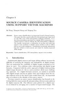
The result can be easily shown by analyzing the Karush-Kuhn-Tucker (KKT) conditions in the solution [9]. This functional relationship is a straightforward nexus between the Lagrange multipliers and the residuals. As the numerical regularization modifies the dual formulation, it necessarily modifies the primal formulation. SpecifFig. 1. Robust cost function for the ically, the consideration of the following SVM-ARMA algorithm. cost function   |e| ≤ ε 0, 1 2 LC (e) = 2γ (14) (|e| − ε) , ε ≤ |e| ≤ γC + ε   1 2 C(|e| − ε) − 2 γC , |e| ≥ γC + ε leads to the following function to be minimized: p q
 1
2 1
2 1
 2 ∗ LC ξk + ξk∗2 + C (ξ , ξ , a , b ) = a + bj + (ξk + ξk∗ ) k k i j P i 2 i=1 2 j=1 2γ k∈I1

k∈I2

(15)

constrained to (4) and (5), where I1 is the set of samples for which ε ≤ |ξk | ≤ ξC , and I2 is the set of samples for which |ξk | > eC (Figure 1). The derivation of the dual problem leads to a functional to be maximized which is slightly different from (12), but it has the same solution. Therefore, the primal function we are actually using is not the one suggested in (3), but rather (15). It can be seen as a robust cost function that allows different error penalties (insensitive, quadratic or linear cost) which can be straightly related to the residuals due to the analytical relationship (13), and the free parameters of the SVM can be tuned according to the statistical nature of the problem. A number of results can be derived from the signal analysis point of view, which are being currently developed.

4

Clinical Application Example

A kind of application where the characteristics of SVM-ARMA are appropriate and potentially useful is the digital, signal-based clinical featuring. If clinical

1110

´ J.L. Rojo-Alvarez et al.

features are to be derived after a signal processing procedure, this method should be as robust as possible. In the present section, an example of clinical featuring is presented for qualitative comparison of the SVM-ARMA with the LS solution. The modeling problem is to establish an LTI system representation for the atrial and the ventricular cardiac electrical functions, from signals that are recorded in implantable defibrillators. The usual healthy cardiac rhythm is known as Sinus Rhythm (SR), and it is represented by an almost periodic cardiac activation in both atrial and ventricular channels (electrograms). If the model is shown to be robust enough, it might be used to establish indexes of cardiac alterations from the SR, although this topic is not studied Fig. 2. Robust cost function for the SVM- here. ARMA algorithm. The digitized atrial and ventricular signals were obtained from an implantable defibrillator in a patient during SR (Figure 2). The sample rate was 128 Hz for both channels. (a) The LS criterion. Samples were divided into two non overlapping subsets for fitting the model and testing, with N = 250 samples (three cardiac cycles) each. The Akaike Information Criterion was used to select the best model order, which was ARMA(1,8) [2](Model 1). (b) The SVM-ARMA algorithm. The following procedure was followed for estimating the free parameters. First, γ = 1 was fixed. An initial SVMARMA(40,40) was previously obtained, as this order was a 25% of the cardiac cycle, and it was considered high enough to embed all the coefficients. With ε = 0 and C = +∞, the coefficients were estimated (Model 2). The wide order was shortened by determining the first coefficients containing the 95% of the coefficients energy, leading to an ARMA(2,13) (Model 3). Then, the optimal value for the free parameters was found by sweeping a range for each of them according to the prediction error on the training samples. A range of values was found proper for ε and C, and a possible set of values were ε = 0.2 and C = 2. Figure 3 shows the impulse responses obtained for the models. The estimated system in (b) exhibits oscillation, due to the extremely high number of coefficients. This situation improves after the moderation of the order in Model 3. The agreement between the SVM-ARMA(2,13) before and after parameter tuning (Model 3 and 4) is evident. The spectral analysis of atrial and ventricular channels, together with the spectral representation of systems in Model 1 and Model 4, are shown in Figure 3. Note that: (a) the SVM spectral response provides an enhanced energy compensation in the band where it is required (4 to 18 Hz); (b) the SVM-ARMA does not distort the low-frequency components (0 to 4 Hz), while LS does.

Support Vector Method for ARMA System Identification

1111

Fig. 3. Left: Impulse responses: (a) Model 1; (b) Model 2; (c) Model 3; (d) Model 4. Right: Frequency domain representation. Up: power spectral densities of atrial and ventricular channels. Down: modulus for Model 1 and Model 4.

Therefore, a first approach to this problem shows the SVM-ARMA exhibiting higher reproducibility and robustness than classical LS estimators. Further, specific analysis is being done on the basis of these findings.

5

Conclusions

A first approach to the SVM-ARMA system identification has been suggested. The role of the numerical regularization has been examined leading to a robust cost functional interpretation. A clinical application example has been developed in order to test the algorithm in comparison with the LS approach. Future work includes the extension to the non-linear system identification problem by using Mercer’s kernels and non-uniform sampling. Also, robust modeling of cardiovascular and hemodynamic biomedical signals is being currently developed.

References 1. Proakis, J.G., Rader, C.M., Ling, F., Nikias, C.L.: Advanced Digital Signal Processing. Macmillan Publishing Company, NY, US, 1992. 2. Ljung, L.: System Identification. Theory for the User. Prentice Hall, NJ, US, 1987. 3. Vapnik, V.: The Nature of Statistical Learning Theory Springer–Verlag, NY, 1995. 4. Sch¨ olkopf, B., Sung, K.: Comparing Support Vector Machines with Gaussian Kernels to Radial Basis Function Classifiers IEEE Trans. on Signal Proc. Vol 45, n 11. 1997. 5. Pontil, M., Verri, A.: Support Vector Machines for 3D Object Recognition. IEEE Trans. on Pattern Anal. and Mach. Intell. Vol. 20, n 6, 1998. 6. M¨ uller, K.R., Smola, A., R¨ atsch, G.R., Sch¨ olkopf, B., Kohlmorgen, J., Vapnik, V.: Predicting Time Series with Support Vector Machines. In Advances in Kernel Methods. Support Vector Learning. MIT Press, MA, USA. 1999. 7. Tikhonov, A.N., Arsenen, V.Y.: Solution to Ill-Posed Problems. V.H. Winston & Sons. Washington, US, 1977. 8. Smola, A.J., Sch¨ olkopf, B.: A Tutorial on Support Vector Regression. NeuroCOLT2 NC2-TR-1998-030,1998. 9. Luenberguer, D.G.: Linear and Nonlinear Programming. Addison–Wesley Pub Co, Reading, MA, 1984