augment some other machines until it becomes 0. Nevertheless, after the production capacity of stage 4 increases, the dual price of stage 6 rises from 0 to 2132,.
Proceedings of the International MultiConference of Engineers and Computer Scientists 2008 Vol II IMECS 2008, 19-21 March, 2008, Hong Kong
Identifying Bottleneck Cells with Goal Programming Yen-Yin Ho, Hsien-Tang Tsai, and Shian-Yang Tzeng
Abstract—In the hi-tech industries the emerging bottleneck(s) will restrict the whole production line and influence the factories’ capability to make money, especially in Taiwan where OEM is the prevail way to earn low margin. In order to solve the problem efficiently, TOC can provide on-going improvement to the work sites. This paper shows how to use goal programming to identify the bottlenecks and the sensitivity analysis is presented. The analysis is illustrated with an empirical case. Index Terms—theory of constraints, Goal programming, bottleneck management.
I. INTRODUCTION In 1980s, American business gradually fell behind in industrial competitiveness. To take it as a mirror, the just-in-time management system which Toyota, a Japanese company, boosted all out is so popular. Therefore, how to enhance productive activity, decrease inventory, and increase market share now became the spotlight from the academic community and business in the United States. Meanwhile, the advent of theory of constraints [1] began to be prevalent. According to theory of constraints (TOC), there are five steps that can provide on-going improvement to the work sites: Step 1. Identify the system constraint(s). First of all, locate the constraints that prevent the organization from achieving the goal and seek out the weakest part of the whole system. Step 2. Decide how to exploit the constraint(s) Find a way to increase the productivity of constraint sources, for example scheduling the workers’ afternoon time break and leaving the machines working nonstop. Don’t haste to purchase or upgrade the current sources. Step 3. Subordinate everything else to the above decision. Do something not to let other activities hinder the productivity of constraint sources. For example, when down time falls because of waiting for materials at bottleneck stages, align other activities to the production activities at bottleneck stages. If the bottlenecks still exist after efforts, go to step 4. If not, go to step 5. Step 4. Elevate the system constraint(s). Increase capacity of production or upgrade to eliminate the constrains or alleviate its influence. Step 5. If, in the previous steps, a constraint has been broken, go back to step 1. Don't let inertia become the constraint. Consistency, permanent improvement can make the system operation reach divinity. Nowadays the increasing output value of hi-tech products is the primary source of Taiwan’s economic growth. Because of the market’s drastic competitiveness and the customer’s various needs, all the life cycles of hi-tech products have been condensed. To fight for market share, rapidly retrieve investment capital, and prepare for the next
ISBN: 978-988-17012-1-3
stage of competition, the exploitation, production, and entering market of new productions always run against time. At the same time the purchase prices of machines are high, and the ratio of depreciation increases steadily. This is a common phenomenon in the hi-tech industries. Under the scenario above, the emerging bottleneck(s) will restrict the whole production line and influence the operation’s ability to make money. Even worse, it may cause massive accumulation of the work in process and ends up overstocking. In order to solve the problem efficiently, TOC can provide a useful framework in the work sites. And, more specific algorithm and calculation are needed to let the production managers to make decisions accurately and efficiently. The objective of this paper is to show that goal programming (GP) can be used to identify the bottleneck of a factory, and the relevant financial figures can be calculated when the real data can be collected accordingly. In section 2, a review of relevant literature is presented. In section 3, research methods are introduced. In section 4, we explore the practicality of the model and collect data with an empirical case. The calculation and result is illustrated in section 5 and finally end with conclusion and discussion. II. LITERATURE REVIEW The bottleneck is defined as a critical resource, which determines the throughput rate and therefore an operation’s ability to make money [2]. And the dominant bottleneck is the resource that has the largest difference between its available and required capacity [3]. How to systematically detect and solve the bottleneck problem with mathematical model is a must to the practical application of production management and academic research. Most of the related researches treat bottlenecks as known variables and skip down to planning schedule [4,5,6,7]. But, it’s not an easy task to identify the bottleneck stages. Practically, those industrial engineers with the site experience can subjectively and precisely locate the bottleneck stages, e.g. a great number of overstocking work in process. But it is hard to estimate how great they could affect, especially the real number of cost and financial impact. Applying what procedures to tackle the problem really requires more accurate analysis. This paper focuses on how to identify the bottleneck stages with goal programming and demonstrate the feasibility of the method we use by making mathematical calculations of a case. The next section will introduce linear programming. III. RESEARCH METHODS Linear programming (LP) is a tool for solving optimization problems. Many practical problems in operations research can be expressed as linear programming problems. Certain special cases of linear programming, such as network flow problems, productivity combination problems, and multicommodity flow problems are
IMECS 2008
Proceedings of the International MultiConference of Engineers and Computer Scientists 2008 Vol II IMECS 2008, 19-21 March, 2008, Hong Kong considered pretty important to derive many researches on specialized algorithms for their solutions. A number of algorithms for other types of optimization problems work by solving LP problems as sub-problems. Ideas from linear programming have inspired many of the central concepts of optimization theory, such as dual, reduced cost, and sensitivity analysis. In operations research, linear programming is heavily used in management problems, either to maximize the income or minimize the cost of a production scheme. Standard form (minimization problem) can be presented as follow:
Or ( maximization problem):
For example, to maximize the objective function, we seek the maximum profit under all the constraints, such as the capacity of machine productions, the working hours of machines, the production capacity to fill the order …etc. Since too many constraints may meet infeasible solutions, to sort it out, we can apply a similar concept of goal programming [8] to add deviational variables to some constraints. Through the values of deviational variables, we can soon realize if it’s an overdone or underdone condition. Then with sensitivity analysis, as dual price is greater than zero, we see that a change in the right-hand side of a constraint will add a change to the objective function. If a constraint has a large positive dual price, we can say that the constraint is the “constraint source”, which is the bottleneck and requires more attention. By the way, applying linear programming can meet the question’s requirement: detect the bottlenecks and seek improvement methods at the next stage. At the following section, we will take a high-tech company as an example and elaborate on it. IV. PROBLEM DESCRIPTION AND DATA COLLECTION In this section, the IC packing industry will be introduced briefly and an empirical case is illustrated. The global IC packaging and testing industry has a keen competition. This paper tries to research how the case company budgets its existing machines and equipment to boost the utility rate, how it plans capital expenditure to update the equipment to make better production processes, and how it improves yield rate to respond the demands of the target market and enhance the enterprise’s competence. IC packaging and testing industry is the back-end part of the IC production process. In Taiwan, it is a labor-intensive industry, and advanced countries such as U.S. and Japan control its core technique and equipments. Generally, IC
ISBN: 978-988-17012-1-3
packaging process has the following features: 1. Customized process Most companies in IC packaging industry are OEM firms, which should manufacture in compliance with customers’ requests, such as specifications, materials, and equipment. 2. Many limitations: During IC packaging process, there are many limitations to maintain product quality and avoid human errors. Those errors include batch control-easily tracing quality problems, material control - different products using different materials, and the parameter limitation of production equipment - the parameter setting of production equipment in accordance with different products and their materials. 3. Short life cycles Electronic products have short life cycles. To maintain its competitive advantage, IC packing tends to develop the model of high pin count and high connection density. 4. Different batch sizes On the same production line, the orders of different batch sizes are commonly manufactured together. Hence, there is no so-called “standard batch material” and all the production batch sizes should meet customers’ expectations. To effectively achieve the production goal, marketing, production management, and production line ought to operate in coordination. Based on the production processes, all sections need to check the gaps between planned production and realized production, review and solve the problems, and then improve the production goal daily. Often the factories face insufficient production capacity because of strong demands. Then it is essential for selling and benefits to locate and break through the bottlenecks on the work stages under the condition of similar weekly orders. According to the on–site engineers’ record, we organize some related variables and obtain the data below (see Table1 and Table 2). Assuming that the total number of orders is the same but the weekly numbers are various, we simulate distinct combinations of 23 products using random numbers to calculate the production capacity of each product and the total profit of the planned goal. Moreover, we conduct sensitivity analysis to observe how the change of right-hand-side numbers affects the objective goal. After numerous simulations, the work stages with constraint resource will be spotted and therefore the undertaker can move on to the evaluation stage of new machine purchase. The random number generator can create all the order combinations q1,q2,…,q23, which are also the decision variables. Next section we will demonstrate the calculation by using LINDO. V. MODEL AND CALCULATION OUTCOMES We apply linear programming to test the feasibility of the model. Model formulation s
IMECS 2008
Proceedings of the International MultiConference of Engineers and Computer Scientists 2008 Vol II IMECS 2008, 19-21 March, 2008, Hong Kong Given: Number of machines Sj j=1,2,…,8 Capacity of each station per hour hij i=1,2,……..23 Price pi
j=1,2,…,8
i=1,2,……..23 Product cost ci i=1,2,……..23 The simulated number of orders
qi
i=1,2,……..23 The LP general function is as follows: Max = Σx i ⋅ (Pi − c i ) − penalty s.t . Σ x i / hij ≤ s j ⋅ 24 ⋅ 7
j = 1,2,...,8
x i = q i + ni − pi
i = 1,2,...,23
ni ⋅ pi = 0 ni , pi ≥ 0
Note: penalty occurs when the deadline of order is missed. Calculation and sensitivity analysis In this section, the production capacity, selling price, product cost, and the number of machines listed above will be introduced into the model and then LINDO program will be executed. After the execution, we can’t find the feasible solution because of too many constraints. To change the constraints, we add deviational variables ni and pi to come up with a compromise solution. The adjusted constraints are as follows: x1=66000+n1-p1; x2=149000+n2-p2; ………………… x23=248000+n23-p23
After the second execution, we may obtain Figure 1. and Figure 2. According to the sensitivity analysis, we find the dual prices of stage 2, 3, 4, 6 are greater than 0, which means if we compromise the right-hand sides, i.e. the working hours of the machines, the objective function, i.e. the benefit, will increase. We can conclude that the stage 2, 3, 4, 6 are bottlenecks under these order combinations. Since order combinations vary, we may further observe which stage is often identified as a bottleneck. Work-site supervisors should pay more attention to those bottleneck stages by increasing the constraint sources such as outsourcing, reusing old machines, prioritizing the arrangement of standby technology repairmen, and adjusting periodical maintenance and repair time [9]. Furthermore, they can purchase new equipment to expand the production and advance the gains. Other simulation outcomes are shown as table 3, and 4.
many changes can be added, we pursue further calculations. Adjusting the constraints in simulation 3 by purchasing a new machine on stage 4, we will get additional 24*7=168 working hours. The outcome of recalculation is shown in table 5. The objective goal (profit) will increase from 12,615,559 dollars per week to 13,356,339 dollars per week. Because the dual price on constraint 4 is still greater than 0, we can augment some other machines until it becomes 0. Nevertheless, after the production capacity of stage 4 increases, the dual price of stage 6 rises from 0 to 2132, which means when some source constraint is loosened, the whole production will elevate. Those products that are not or less manufactured due to the bottleneck on stage 4 now are put into consideration to augment them. This change may induce a new bottleneck on another stage. That is, bottlenecks are floating. Through 3 simulations, generally, stage 4 requires more attention. Providing we have 50 -week simulations of order combinations, the bottleneck stage must be more identifiable. Our conclusions are as follows: 1. LP can be applied to identify bottlenecks. 2. Checking the dual prices on LINDO output can exploit the capacity of constraint resources. 3. Bottlenecks are floating. Some new bottlenecks will be brought up along with some improved bottleneck. 4. With cost benefit analysis, decision makers have more objective information to decide whether to buy new machines or to buy what kind of machines. 5. When focusing on the right-hand side (e.g. machine working hours), we can’t ignore the possibility of left-hand side improvement, for example decreasing the malfunction time and wait time. We can further enhance mobility and production. That is, sometimes, it is better in improving LHS rather than RHS However, there are some limitations in this study. First, we have only simulated the order combinations 3 times, which can be bettered to 50 times. Second, the assumptions such as the fixed cost and price and the known production capacity don’t conform to the experience in the industry, and it still has great room for improvement. If fuzzy theory can be used to randomize the variables above, it will be more persuasive. Linear programming was rarely applied to identify bottlenecks in early work [10]. It deserves further development.
VI. CONCLUSION AND DISCUSSION From the outcome of section above, we find stage 4 has had positive dual prices three times during simulating. In other words, a change in the right-hand side of constraint 4 (machine working hours), will accordingly contribute 2562, 3680, 5325 dollars to the objective goal (profit). As for how
ISBN: 978-988-17012-1-3
IMECS 2008
Proceedings of the International MultiConference of Engineers and Computer Scientists 2008 Vol II IMECS 2008, 19-21 March, 2008, Hong Kong
References Goldratt, E.M., and Cox, J.(1992), The Goal, 2nd revised ed., North River Press: Croton-on-Hudson, NY. [2] Chakravorty, S.S. and Atwater J.B. (2006), Bottleneck management: theory and practice, Production Planning & Control, Vol. 17 Issue 5, p441-447. [3] Aryanezhad, M.B. and Komijan, A.R. (2004), An improved algorithm for optimizing product mix under the theory of constraints, International Journal of Production Research, Vol. 42 Issue 20, p4221-4233 [4] Lee, G., Kim, Y., and Choi, S. (2004), Bottleneck-focused scheduling for a hybrid flowshop. International Journal of Production Research, 42(1): 165-181. [5] Koh, S.G., Koo, P.H., Ha, J.W., and Lee, W.S. (2004), Scheduling parallel batch processing machines with arbitrary job sizes and incompatible job families. International Journal of Production Research, 42(19): 4091-4107. [6] Wang, S., and Sarker, B.R.(2002), Locating cells with bottleneck machines in cellular manufacturing systems. International Journal of Production Research, 40(2): 403-424. [7] Wu, H.., & Yeh, M. (2006), A DBR scheduling method for manufacturing environments with bottleneck re-entrant flows. International Journal of Production Research, 44(5): 883-902.. [8] Charnes, A. and Cooper, W.W. (1961), Management Models and Industrial Applications of Linear Programming, New York: Wiley and Sons. [9] Goldratt, E.M., and Fox, R.E. (1986), The Race, North River Press: Croton-on-Hudson, NY. [10] Mabin, V. J., and Gibson, J. (1998), Synergies from spreadsheet LP used with the theory of constraints - a case study. Journal of the Operational Research Society, 49(9): 918-927. [1]
Table 1. The no. of machines on each stage and their Capacity(9 stages) Codename
The Number of machines
The codename Weekly capacity for each of capacity machine
m1
D/B=16
mp1
49862
m2
ASM=98
mp2
701672
m3
K&S=104
mp3
38130
m4
T/M=20
mp4
41552
m5
M/K=4
mp5
49862
m6
O/V=1
mp6
33997
m7
D/J=6
mp7
31164
m8
T/P=2
mp8
62328
m9
T/F=10
mp9
25970
Table 2. Selling Prices and Costs(23 categories) Price codename
Selling price (dollars)
p1
20.07
c1
17.45
p2
20.07
c2
17.45
p3
27.60
c3
24.00
p4
40.15
c4
34.91
p5
27.60
c5
24.00
p6
62.73
c6
54.55
p7
40.15
c7
34.91
p8
50.18
c8
43.64
p9
50.18
c9
43.64
p10
40.15
c10
34.91
p11
62.73
c11
54.55
p12
80.29
c12
69.82
p13
27.60
c13
24.00
p14
40.15
c14
34.91
p15
50.18
c15
43.64
p16
50.18
c16
43.64
p17
62.73
c17
54.55
ISBN: 978-988-17012-1-3
The codename product cost(dollars) Of product cost
Table 3 Scenario analysis (1) Stage1 Stage2 Stage3 Stage4 Stage5 Stage6 Stage7 Stage8 Slack 0 5137 113 0 284 26 125 64 Dual price 2269 0 0 3680 0 0 0 0 Table 4 Scenario analysis (2) Stage1 Stage2 Stage3 Stage4 Stage5 Stage6 Stage7 Stage8 Slack 9 795 0 0 303 65 132 267 Dual price 0 0 79 5325 0 0 0 0 Table 5 Scenario analysis (3) Stage1 Stage2 Stage3 Stage4 Stage5 Stage6 Stage7 Stage8 Slack 2 1405 0 0 288 0 124 162 Dual price 0 0 376 3147 0 2132 0 0
Global optimal solution found at iteration: 28 Objective value: 0.2064041E+08
Variable X1 X2 X3 X4 X5 X6 X7 X8 X9 X10 X11 X12 X13 X14 X15 X16 X17 X18 X19 X20 X21 X22 X23
Value 0.000000 0.000000 0.000000 0.000000 0.000000 13206.85 0.000000 0.000000 0.000000 0.000000 850666.2 982159.8 0.000000 0.000000 0.000000 0.000000 0.000000 0.000000 837332.4 0.000000 0.000000 0.000000 0.000000
Reduced Cost 3.494317 3.494317 3.518304 3.004749 3.515462 0.000000 2.764513 1.020630 6.312985 2.736773 0.000000 0.000000 2.706171 5.421432 9.808165 4.245189 0.6736439 1.256878 0.000000 0.1758795 0.2161242 0.3064664 4.368446
Figure 1. the Feasible Solutions of LP
Row Slack or Surplus Dual Price 1 0.2064041E+08 1.000000 2 319.5857 0.000000 3 0.000000 279.1399 4 0.000000 289.8852 5 0.000000 2562.603 6 294.7730 0.000000 7 0.000000 5809.916 8 142.6226 0.000000 9 122.4750 0.000000 Figure 2. Sensitivity Analysis
IMECS 2008