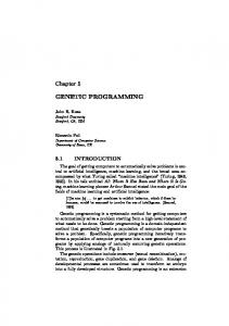
Genetic programming provides a way to solve such complex optimization
problems. In this work, the use of genetic programming to identify the input
variables, ...
Fuzzy Sets and Systems 113 (2000) 333–350 www.elsevier.com/locate/fss
Identifying fuzzy models utilizing genetic programming Andreas Bastian Electronic research, Brie�ach. 1776, Volkswagen AG, 38436 Wolfsburg, Germany Received August 1997; received in revised form March 1998
Abstract Fuzzy models o�er a convenient way to describe complex nonlinear systems. Moreover, they permit the user to deal with uncertainty and vagueness. Due to these advantages fuzzy models are employed in various elds of applications, e.g. control, forecasting, and pattern recognition. Nevertheless, it has to be emphasized that the identi cation of a fuzzy model is a complex optimization task with many local minima. Genetic programming provides a way to solve such complex optimization problems. In this work, the use of genetic programming to identify the input variables, the rule base and the involved membership functions of a fuzzy model is proposed. For this purpose, several new reproduction operators are c 2000 Elsevier Science B.V. All rights reserved introduced. Keywords: System identi cation; Fuzzy modeling; Genetic programming
1. Introduction By the term system an object in which variables of di�erent kinds interact and produce observable signals is described. When interacting with a system, a sound understanding of how the variables of that system relate to each other is usually of major importance. We will refer to such a relationship as a model of the system. Clearly, not every system can be exactly represented by a mathematical model. Take for instance the task of modeling a driver backing up a car. The closer we look at this problem, the more we realize the di�culty of writing down a rather concise mathematical model. Interestingly, we actually can describe the action of this driver in terms of simple linguistic rules, as it was done for example in [1]. Fuzzy logic provides a convenient method to implement such knowledge into
computers. This logic is the concept of fuzzy sets [18] incorporated into the framework of multivalued logic. The models expressed by this concept are called fuzzy models. We distinguish between relational fuzzy models and rule based fuzzy models. Since the rule based model is the most often employed one, in this work we will focus on this model type. The development of fuzzy models began very early. As a matter of fact, one can view the very rst fuzzy controller by Mamdani (and Assilian) [11] as a fuzzy model of the human operator’s control actions. Today, fuzzy models are widely employed. They cover a wide range of applications: from the control of an unmanned helicopter [14] to the judgment of river water [7]. Unfortunately, the identi cation of fuzzy models is a very complex task that comprises the identi cation of (a) the input and output variables, (b) the rule base, (c) the membership functions and (d) the mapping
c 2000 Elsevier Science B.V. All rights reserved. 0165-0114/00/$ - see front matter PII: S 0 1 6 5 - 0 1 1 4 ( 9 8 ) 0 0 0 8 6 - 4
334
A. Bastian / Fuzzy Sets and Systems 113 (2000) 333–350
parameters. Thus, we face an optimization task with many local minima. The complexity of this task was shown for instance in [5]. Today, we can nd a large amount of fuzzy model identi cation approaches. Yet, most of those proposed methods are simply identifying the membership functions of a prede ned rule base. In other words, an optimization of the membership function is performed. If also the rule base has to be identi ed, the optimization becomes more complex, since the amount of the parameters to be optimized varies with the size of the rule base. For those two identi cation cases, neural networks have proven to be very e�ective optimization tools. Especially when the fuzzy model is incorporated into the neural network structure, the learning algorithms of the neural networks perform very good. One example is the local linear model tree (LOLIMOT) algorithm [13]. This neuro-fuzzy approach consists of an upper level that determines the input partition, while a lower level estimates the parameters. Another neuro-fuzzy approach was proposed in [10]. Here, a two-phase neural network was proposed that combines unsupervised learning and supervised gradient descent learning to construct the rule nodes and optimize the membership functions of the node terms. Notice that those two algorithms assume that the “right” input variables are already known in advance. Thus, no good model can be identi ed if “wrong” input variables are o�ered to the algorithms described above. Unfortunately, especially in real life applications, we are often faced with a fast number of possible input variables. Here, an algorithm that identi es also the input variables of the model would be very useful. Scanning through the literature, we will not encounter many fuzzy model identi cation approaches that identify the input variables, the rule base and the involved membership functions. The approach described in [3] starts by clustering the data using the fuzzy c-means algorithm [6]. Therefore the modeling result depends very much on the employed cluster validity function. Since the selection of the cluster validity function is not always trivial, this approach is somehow limited in its use. Moreover, the top-down nature of the algorithm tends to lead the optimization into one of the nearest local minima. Another approach that also identi es identi es the input vari-
ables, the rule base and its membership functions was described in [15], however, this modeling approach was designed for quantitative modeling, thus the numerical accuracy of the fuzzy model is not very good. Moreover, also this approach depends very heavily on the fuzzy c-means algorithm. In view of the fact that fuzzy models are becoming increasingly popular for modeling complex technical systems there is a need for an identi cation method that identi es the input variables, the rule base and the involved membership functions. In this work, a fuzzy model identi cation method based on genetic programming [9] is proposed. Due to the parallel nature of the evolutionary algorithm, the possibility to reach a global minimum is rather high. The proposed method is of universal nature, thus there is no limitation in its usage. This paper is organized as follows: in Section 2 the basic de nitions of the to be identi ed fuzzy models are presented. In Section 3 the identi cation approach is discussed in detail. In Section 4 an application examples is given, followed by the conclusion in Section 5.
2. Fuzzy models 2.1. Basic de nitions The fuzzy models used in this work are based on the compositional rule of inference. Such a model consists of three main blocks as shown in Fig. 1. In the input block the crisp input values are transformed into fuzzy sets. Usually those fuzzy sets are in form of singletons since they are natural and easy to implement. This transformation is named fuzzi cation. The inference block contains the rule base consisting of a certain amount IF–THEN rules. The fuzzi ed data are passed to this block and are matched to each rule antecedent. The result of this matching is the degree of membership. When an antecedent contains several conditions then the overall degree of match of this antecedent has to be determined rst. The sentence connectives in the antecedent, e.g. the connective AND, are usually implemented as fuzzy conjunctions in a Cartesian product space in which the variables take values in di�erent universes of discourse. Commonly used aggregation operators for the
A. Bastian / Fuzzy Sets and Systems 113 (2000) 333–350
335
Fig. 1. Computational structure of a fuzzy model.
connective AND are the minimum and the product operators. Subsequently the meaning of the IF–THEN rule is determined using the implication function. To represent the output values of all rules, a fuzzy set of output values is obtained using the compositional operator. One commonly used operator is the max-operation. To obtain a crisp output, the resulting fuzzy value is mapped back to the crisp domain in the output block. This mapping is called defuzzi cation. One common defuzzi cation strategy is the center of gravity method: P w�C (w) ; zo = P �C (w)
(1)
Fig. 2. Membership functions.
where Ri is the ith rule, xj are the j linguistic input variables, y is the linguistic output variable, and Aij and Bi are the linguistic values of those variables. For simplicity Eq. (2) is rewritten as Ri : IF (x is Ai ) THEN (y is Bi );
(3)
where �C is the membership function of the inferred consequence C which is pointwise de ned for all w in the universe of discourse W . In respect of the consequence part of an IF–THEN rule, there are two widely employed types of rules: the M-type by Mamdani [11], and the TSK-type by Takagi, Sugeno and Kang [16]. In this work we will only consider the M-type of fuzzy rule where each consequence is a linguistic value. The fuzzy rules create a partitioning of the input spaces, with an linguistic output value being assigned to each of those spaces. For a single output and multiple input system the rules have the form:
where x = (x1 ; : : : ; xn ), and A = (A1 ; : : : ; An ). In this work, trapezoidal membership functions are employed to represent the input terms. The trapezoidal membership function Tz: U ∈ [0; 1] is a function de ned as follows: 0; u¡a; a6u6b; (u − a)=(b − a); b6u6c; Tz(u; a; b; c; d) = 1; (d − u)=(d − c); c6u6d; 0; u¿d:
Ri : IF (x1 is Ai1 ) AND (x2 is Ai2 ) · · · AND (xn is Ain )
Fig. 2 pictures this de nition. This notation is very convenient since it allows the algorithm to freely choose between the type of membership function.
THEN (y is Bi );
(2)
(4)
336
A. Bastian / Fuzzy Sets and Systems 113 (2000) 333–350
Fig. 3. Fuzzy model identi cation [13].
The output terms are represented by singleton membership functions, de ned as follows: ( 0; u 6= 1; S(u; a) = (5) 1; u = a: In this work only complete rule bases are considered. A rule base is said to be complete when any combination of input values results in an appropriate output value. Therefore, the number of rules of a fuzzy model can always be deducted from the number of input variables and the corresponding number of terms. For example: a fuzzy model with two input variables where the input X consists of two terms and the input Y consists of three terms has a total of six fuzzy rules. 2.2. Fuzzy system identi cation Fuzzy system identi cation is the process of identifying the structure and the parameters of a fuzzy model. This process can be de ned as shown in Fig. 3. The structure identi cation of a fuzzy model consists of the input variable identi cation and the rule identi cation. The input variable identi cation is the identi cation of the input variables of the model. The rule identi cation consists of (a) the identi cation of the rule type used by the fuzzy model to represent a given input-output data relation, and (b) the identi cation of the rule structure. The latter is the process of selecting the input and output variables involved in each individual rule, and determining the number
Table 1 The common fuzzy model identi cation cases Identi cation
Input variables
Rule structure
Rule parameters
Mapping parameters
Case Case Case Case Case Case Case Case
X X X X
X X
X X X X X X X X
X
1 2 3 4 5 6 7 8
X X
X X X
of rules. The parameter identi cation consists of (a) the rule parameter identi cation, and (b) the mapping parameter identi cation. The rule parameters are all the parameters related directly to the interpretation of a fuzzy rule, as there are the membership functions, the aggregation operator and the implication function. The mapping parameters are the parameters related to the mapping of a crisp set to a fuzzy set, and vice versa. In view of this distinction, we can distinguish between several identi cation cases. In the Table 1 the most common cases found in the literature are displayed. A concise treatment about fuzzy system identi cation can be found in [2]. The most common identi cation is Case 8 where usually only the membership functions of a given rule base are identi ed. As one can see, Case 1 subsumes all other identi cation cases. In this work we will employ genetic programming for the Case 4 identi cation task.
A. Bastian / Fuzzy Sets and Systems 113 (2000) 333–350
337
Fig. 4. Cycle of reproduction.
3. Genetic programming for fuzzy system identiÿcation
5. If necessary, mutate the new individual. 6. Repeat from Step 3 until a new population (new generation) is established.
3.1. The basic paradigm It has been shown in several publications, e.g. [4,17], that genetic programming is a very powerful tool for system identi cation when only little about the underlying structure in the data is known. Therefore, in this work the usage of genetic programming for the identi cation of fuzzy models is proposed. Genetic programming [9] can be regarded as an extension of the common GA [8]. Like the GA, it combines a survival the ttest optimization strategy with a structured yet randomized information exchange; and since the search is conducted from a population, even large search spaces can be covered quickly. Its cycle of reproduction is shown in Fig. 4. In essence, the evolution of an arti cial population can be simulated as follows: 1. Generate an initial population. 2. Evaluate the individuals and assign tness values to them. 3. Use a biased random process to select (usually two) individuals for reproduction. 4. Perform the reproduction.
3.2. Some basic de nitions Deÿnition 1. The coded information in an individual is named its structure. It consists of tree-like arranged nodes. In this work several basic nodes are used: (a) P-nodes containing parameters, (b) V-nodes containing variables, (c) A-nodes containing arithmetic operators, (d) T-nodes containing the number of terms of a linguistic variable, and (e) M-nodes containing fuzzy membership functions. The structure shown in Fig. 5 consists of two A-nodes containing the division and subtraction operators, two V-nodes containing the parameters X and Y , and one P-node containing the value 4. This structure is named a functional structure since it contains a function. Such functional structures are decoded using the simple rule (left branch or node) (execute preceding A-node) (right branch or node):
(6)
A. Bastian / Fuzzy Sets and Systems 113 (2000) 333–350
338
where T is the node type, n the number of its input connections to it, m the number of its output connections, V its node vector, x and y are the sets of permitted node types of the inputs and the outputs. 3.3. Mechanisms of reproduction
Fig. 5. A structure containing the function f(X; Y ) = X=(Y − 4):
This rule is applied bottom-up, starting from the left most terminal node. Using this rule the structure is decoded as follows: Eq. (6) is applied starting from the left most terminal node, in this case the V-node “X ”, resulting in: f(X; Y ) = X=(right branch):
(7)
Decoding the left branch according to the general rule given in Eq. (6) results in right branch = Y − 4:
(8)
Inserting (8) into (7) yields the function f(X; Y ) =
X : Y −4
(9)
If a structure only consists of P- and A-nodes it is called a parameter structure. Here, the decoded structure is a constant. We will use such parameter structures to code fuzzy membership functions. For real world applications, the universe of discourse of every node type has to be restricted. For this purpose, so-called node vectors are introduced. A node vector contains the permitted contents of a node. For example: the P-node vector Vp = {0; 1; 2; 3; 4; 5}
(10)
contains six possible node contents. To ensure that every individual contains a comprehensible solution, the relations between the di�erent node types have to be de ned. For this purpose socalled node protocols are de ned for each node type: P(T) = { n; m; V | x ∈ (permitted types); y ∈ (permitted types)};
(11)
3.3.1. The cloning operation The cloning operation ensures that a certain amount of individuals with outstanding tness values will survive and appear in the next generation. This measure prevents the algorithm from loosing the best found solution. Usually, the best individual of a generation is copied into the following generation. This operation is often referred to as elitist strategy. 3.3.2. The crossover operation This operation is producing an o�spring that inherits some of the characteristics of its parents. For a better understanding, let us rst observe the structure of an individual. The individual in Fig. 6 presents a fuzzy model with one output Z and two inputs X1 and X2 where the input X1 consists of the two terms A1 and A2 and the input X2 consists of the three terms B1 , B2 and B3 . Thus, the rule base of this fuzzy model contains six rules. Since each rule is de ned to has its own output, there are six output terms C1 ; : : : ; C6 . The very rst node is the so-called main node. Its only function is to connect all branches of the tree. This main node is followed by three V-nodes containing the two inputs and the output. Each input V-node is followed by a T-node containing the number of terms the preceding input variable has. Each T-node is followed by M-nodes representing the membership functions. Each M-node is connected to four parameter structures representing the parameters of the membership function. In this example the membership function A1 is the function Tz(x; 0; 0; 2; 2:66) and the output singleton C1 is the function S(z; 7:5). In a crossover operation two parents are selected using the roulette wheel method [8]. The new individual is produced by copying the rst selected parent and subsequently swapping some parts of its structure with equivalent parts from the structure of the second parent. For this purpose, in the structure of the rst selected parent (also called dominant parent) one random node
A. Bastian / Fuzzy Sets and Systems 113 (2000) 333–350
339
Fig. 6. An individual containing a fuzzy model.
Table 2 Node types and the related crossover operations Node type
Crossover operation(s)
V-node
General variable crossover or local variable crossover General term crossover or local term crossover Membership function crossover Node crossover or branch crossover
T-node M-node P- or A-node
is selected by using a uniform probability distribution. This node is named the crossover node. Having selected the crossover node a suitable crossover operation can be carried out. Table 2 shows the di�erent crossover operations in dependency of the crossover nodes. The general variable crossover operation swaps whole input or output variables including the involved membership functions. Note that an input variable can not replace an output variable, and vice versa. This operation is performed as follows: (i) The rst selected parent is the dominant one. The other parent is the recessive one.
(ii) If the crossover node is an input variable select randomly one input V -node from the structure of the recessive parent. Otherwise select the output V-node. (iii) Cut away the branches with the crossover nodes. (vi) Copy the rest of the dominant parent and insert the branch cut o� from the recessive parent. (v) If due to the rule base adjustment additional output membership functions are needed, copy the required output membership functions from the recessive parent. Otherwise delete the unnecessary membership functions. The result is the o�spring. Example 1. The dominant parent is a fuzzy model with the input variables X1 and X2 , consisting of four fuzzy rules, namely: IF (X1 is A1 ) AND (X2 is A3 ) THEN (Z is B1 ) IF (X1 is A2 ) AND (X2 is A3 ) THEN (Z is B2 ) (12) IF (X1 is A1 ) AND (X2 is A4 ) THEN (Z is B3 ) IF (X1 is A2 ) AND (X2 is A4 ) THEN (Z is B4 )
340
A. Bastian / Fuzzy Sets and Systems 113 (2000) 333–350
with the membership functions de ned as follows: A1 = Tz(x; 4:66; 5; 10; 20); A2 = Tz(x; 10; 30; 40; 50);
Given that the general variable crossover operation is selected. The crossover node of the dominant parent is the V -node X2 , and that of the recessive parent is the V -node X3 . The resulting o�spring is the fuzzy model with the following rule base:
A3 = Tz(x; 10; 10; 10; 20); A4 = Tz(x; 10; 45; 50; 50); B1 = S(z; 5);
IF (X1 is A1 ) AND (X3 is C3 ) THEN (Z is B1 ) (13)
IF (X1 is A2 ) AND (X3 is C3 ) THEN (Z is B2 )
B2 = S(z; 10);
IF (X1 is A1 ) AND (X3 is C4 ) THEN (Z is B3 )
B3 = S(z; 15);
IF (X1 is A2 ) AND (X3 is C4 ) THEN (Z is B4 )
B4 = S(z; 5);
IF (X1 is A1 ) AND (X3 is C5 ) THEN (Z is D5 )
The recessive parent is a fuzzy model with the input variables X1 and X2 , consisting of six fuzzy rules, namely:
IF (X1 is A2 ) AND (X3 is C5 ) THEN (Z is D6 )
(16)
D5 = S(z; 13);
with the membership functions as de ned in the Eqs. (13) and (15). The local variable crossover operation resembles the general variable crossover operation. The input variables are again swapped. However, in this case the partitioning of the previous variable is kept. In other words, an input variable takes over the parameters of another one. The general term crossover operation swaps the partition of input variables including the involved membership functions, while in the local term crossover operation the membership functions are kept. Thus, this operation is changing the number of terms of one variable. If the new partitioning requires additional terms, they are copied from the other parent, otherwise unnecessary membership functions are deleted. The membership function crossover operation swaps whole membership functions of terms. The node crossover operation is changing the parameters of the membership by swapping single nodes of the parameter structures representing the parameters of the membership function, while the branch crossover operation is changing the parameters of the membership by swapping whole branches of the parameter structures of the parents. A detailed description about those crossover operations can be found in the Appendix. Note that during all operations in this work the algorithm ensures that for a membership function Tz(X; a; b; c; d):
D6 = S(z; 30):
a¿b¿c¿d
IF (X1 is C1 ) AND (X3 is C3 ) THEN (Z is D1 ) IF (X1 is C2 ) AND (X3 is C3 ) THEN (Z is D2 ) IF (X1 is C1 ) AND (X3 is C4 ) THEN (Z is D3 ) (14) IF (X1 is C2 ) AND (X3 is C4 ) THEN (Z is D4 ) IF (X1 is C1 ) AND (X3 is C5 ) THEN (Z is D5 ) IF (X1 is C2 ) AND (X3 is C5 ) THEN (Z is D6 ) with the membership functions de ned as follows: C1 = Tz(x; 2; 2; 12:333; 20); C2 = Tz(x; 4; 5; 6; 10); C3 = Tz(x; 10; 10; 30; 30); C4 = Tz(x; 3; 45; 50; 60); C5 = Tz(x; 10; 15; 20; 20); D1 = S(z; 1); D2 = S(z; 13); D3 = S(z; 12); D4 = S(z; 93);
(15)
(17)
A. Bastian / Fuzzy Sets and Systems 113 (2000) 333–350
341
Fig. 7. The branch crossover operaton.
by swapping the parameter structures representing those membership function parameters. Also if a = b = c = d, then a new parameter structure d¿c is created.
sen for the crossover operation. The crossover nodes are marked with boxes. The dominant parent has the term A1 A1 = Tz(x; 4:66; 5; 10; 20):
Example 2. The branch crossover operation is to be performed on the two individuals from the previous examples. Fig. 7 shows the parameter structures cho-
(18)
The resulting o�spring is shown in the right part of the Fig. 7. It is a copy of the dominant parent with a
342
A. Bastian / Fuzzy Sets and Systems 113 (2000) 333–350
Table 3 Node types and the related mutation operations Node type
Mutation operation(s)
V-node T-node M-node P- or A-node
Variable mutation Term mutation Membership function mutation Node mutation or branch mutation
modi ed term A1 A1 = Tz(x; 28; 5; 10; 20):
(19)
Since the term A1 as de ned in Eq. (19) is violating the protocol of a membership function as de ned in Eq. (17), the parameters of the membership function have to be swapped, resulting in the following term: A1 = Tz(x; 5; 10; 20; 28):
(20)
3.3.3. The mutation operation The mutation is a mechanism to modify reproduced children in order to enlarge the variation in the population. If an o�spring is selected to undergo mutation, in its structure one random node is selected by using a uniform probability distribution. This node is named the mutation node. As in the case of the crossover operation, the mutation operation depends on the mutation node type. Table 3 shows the possible mutation operations. The variable mutation operation changes the input variables of the o�spring. This operation is performed as follows: (i) Select randomly a V-node from the de ned V -node vector. (ii) Swap the mutation node with the selected V-node. (iii) If additional output membership functions are needed, generate randomly the required membership functions. Otherwise delete the unnecessary membership functions. The term mutation operation changes the partition size of an input variable. The membership function mutation operation modi es the membership functions of a term. The node mutation aims at introducing new nodes into the parameter structures. The branch mutation operation reduces or extends the size of the parameter structure by cutting away
branches or adding a new branch. This operation helps the population to develop new generations stemming from good individuals. A detailed description about those crossover operations can be found in the Appendix. Example 3. The node mutation operation is to be performed on the o�spring from the previous examples. The left part of the Fig. 8 shows the parameter structure of the o�spring before mutation. It has the term A1 A1 = Tz(x; 4:66; 5; 10; 20):
(21)
One node is randomly selected for mutation. This mutation node is marked with a box. The mutated o�spring is shown on the left side of the Fig. 8. The resulting o�spring is a copy of the dominant parent with a modi ed term A1 A1 = Tz(x; 15:33; 5; 10; 20):
(22)
As in the previous example, the parameters of the term A1 have to be swapped. The modi ed term is A1 = Tz(x; 5; 10; 15:33; 20):
(23)
3.4. Applying the algorithm In view of the large search space and the large amount of reproduction possibilities, an e�cient evolution mechanism has to be found in order to limit the computing time as well as the population size. First, the probability to perform certain crossover is biased as shown in Table 4. Those are the so-called crossover ratios. The probability to perform certain mutation operations is shown in Table 5. Those are the so-called mutation ratios. The ratios shown in the Tables 4 and 5 are determined after a series of identi cation experiments. One of those experiments is described in the following: to investigate the in uence of the crossover ratios, the three di�erent ratio sets shown in Table 6 were de ned. The mutation ratios are the ones de ned in Table 5. A data set consisting of 250 training data was generated using a prede ned two input single output fuzzy model consisting of four rules. Data of two additional input variables were randomly generated and added to
A. Bastian / Fuzzy Sets and Systems 113 (2000) 333–350
343
Fig. 8. The node mutation operation.
Table 4 Probability of the crossover operations to be selected Crossover method
General variable
Local variable
General term
Local term
Membership function
Node
Branch
Probability
0.05
0.05
0.15
0.15
0.1
0.25
0.25
this data set. The task was to identify a model based on those training data. Thus, the task consists of the identi cation of (a) the input variables, (b) the number of terms, and (c) the membership functions. The algorithm was restricted as follows: (1) the maximum number of model inputs was set to three, and (b) the maximum number of terms was set to three. The identi cation was terminated after 1000 generations. The population size was set to 1000 individuals. The tness of an individual is determined by calculating a biased mean squared error of the fuzzy model: Pm MSE =
i=1 (yi
m
− wi )2
+k
r ; rmax
(24)
where m is the number of data within the support of the antecedent fuzzy sets of the ith rule, y the desired output value, w the result of the decoded individual, k a
Table 5 Probability of the mutation operations to be selected Mutation method
Variable
Term
Membership formula
Node
Branch
Probability
0.05
0.2
0.15
0.3
0.3
constant, r the number of rules used by the individual, and rmax the maximum amount of possible rules. The in uence of the crossover ratio set on the convergence speed of the algorithm is shown in Fig. 9. As shown in this gure, the algorithm with the ratio set 1 yields the best result. After only 300 generations the correct input variables and number of terms was found. The correct membership functions were retrieved after additional 311 generations. Using the ratio set 2, the algorithm is favoring the term crossover operations. Although the algorithm quickly identi ed
A. Bastian / Fuzzy Sets and Systems 113 (2000) 333–350
344
Table 6 Three ratio sets used by the identi cation algorithm Cross over method
General variable
Local variable
General term
Local term
Membership function
Node
Branch
Ratio set 1 Ratio set 2 Ratio set 3
0.05 0.1 0.2
0.05 0.1 0.2
0.15 0.25 0.2
0.15 0.25 0.2
0.1 0.1 0.1
0.25 0.1 0.05
0.25 0.1 0.05
Fig. 9. In uence of the reproduction ratios on the convergence speed.
the right input variables, due to badly de ned membership functions it took over 800 generations until a model with a rather good t to the data was identi ed. Even though this model consisted of four rules, the correct membership parameters could not be identi ed. The ratio set 3 is favoring the term and the variable crossover operations. The slow convergence shown in Fig. 9 is caused by the poor parameter optimization capability of the algorithm. This nal model consisted of three input variables with 12 rules. This experiment shows the signi cance of the choice of the reproduction ratios. The results of the other experiments carried out to verify the selection of the crossover ratio set are summarized in Table 7. The table is read as follows: rst, the dimension of the single output fuzzy model used to generate the training data is described. In case 1, the fuzzy model consists of 2 inputs where each input consists of three terms. In the following column, the average number of generations needed to achieve a MSE¡100 in three runs is displayed for each ratio set. The population size is again limited to 1000 in-
dividuals. As in the previous experiment, the data of two additional input variables were randomly generated and added to this data set. As one can see, the results continue the trend shown in the rst experiment. Since the identi cation of fuzzy membership functions is a complex optimization task with many local minima, the initialization of the membership function parameters has a huge impact on the convergence, as it was shown in [5] where a modi ed genetic algorithm identi ed fuzzy membership functions. Like it was done in [5], in this work three initialization methods were compared: (a) random initialization, (b) fuzzy C-means based initialization, and (c) mean value initialization. In the random initialization, the parameter structure is randomly generated as described in the previous section. The only additional measure ensures that the membership function parameters are related as described in Eq. (17). In the second initialization method the fuzzy C-means clustering algorithm [6] is used to calculate
A. Bastian / Fuzzy Sets and Systems 113 (2000) 333–350 Table 7 Result of various test problems Identi cation problem 2 input variables 3 × 3 rule base 2 input variables 2 × 5 rule base 1 input variables 5 rules
Number of generation Ratio set 1
Ratio set 2
Ratio set 3
656
770
1512
637
812
1704
701
743
2139
the cluster centers of the data. Because the maximum number of terms is xed, three cluster centers are calculated for each input variable. Using those cluster centers the parameter structures are generated as follows: 1. Each calculated cluster center is approximated by a simple parameter structure. 2. Those parameter structure are de ned to be the core of the membership function. The other parameters of the membership functions are set such that the whole universe of discourse of that input variable is covered by membership functions. 3. The other individuals of the initial population are obtained by modifying those ten individuals using the branch mutation operation. 4. The singleton functions of the output variable is constructed by projecting the core of the rst input variable to the output variable. The result is again approximated by a simple parameter structure. The last initialization method is the so-called meanvalue initialization. In this method, each input variable range is divided into equal three sections. The center value of each section is de ned to be the core of the membership function. Using those mean values the membership functions are de ned as it was done with the cluster centers. Using the reproduction ratios shown in the Tables 4 and 5 the identi cation of the fuzzy model described above is performed again with those three initialization methods. The result of this experiment is displayed in Fig. 10. As one can see, the second initialization method yields superior results. Therefore in this work the fuzzy C-means based initialization is employed.
345
Further analysis of the identi cation process showed that the parameter structure optimization is crucial for the convergence. Although in many cases the algorithm did identify the correct input variables in a very early stage of the identi cation, the convergence was very slow due to the slow identi cation of the membership parameters, and in some cases the algorithm even terminated with falsely identi ed models. As a solution to this problem, a local optimization of the membership functions was carried out for each individual using the downhill simplex method proposed by Nelder and Mead [12]. For this purpose, one P-node of the core of each membership function is optimized for a certain amount of optimization steps. After the optimization, those nodes are replaced by the most suitable nodes in the prede ned P-node vector. 3.5. The program ow The simpli ed program ow of the algorithm is as follows: 1. Generate the initial population. 2. Compute the tness of the population and sort the population according to the tness. 3. If the tness of the best individual is less than 0.001, go to Step 11. 4. Clone the best individual. 5. Select the parents for reproduction using the roulette-wheel method. Randomly select the crossover operation according to the crossover ratios and breed the o�spring. 6. Decide whether or not the o�spring has to undergo mutation. The mutation rate is set to be 0.1. If no mutation is necessary, go to Step 11. 7. Randomly select the mutation operation according to the mutation ratio and mutate the o�spring. 8. If the number of generation¿100 then optimize the parameter structures of the individuals using the downhill simplex method. This optimization is performed for 100 steps. 9. Repeat the algorithm from Step 5 until the new population is established. 10. Repeat the algorithm from Step 2 until 2000 generations are reached. 11. Print out the nal report, save the results and terminate the algorithm.
346
A. Bastian / Fuzzy Sets and Systems 113 (2000) 333–350
Fig. 10. In uence of the initialization method.
4. Application example In this section the proposed algorithm is employed to identify a more complex fuzzy model. For this purpose a fuzzy model with two inputs and one output is constructed. The membership functions of the inputs are displayed in Fig. 11. Using this fuzzy model a data set consisting of 300 data sets were created. Three randomly generated dummy input variables were added to the training data. Thus, the data consisted of ve input variables and the output variable. 250 data sets were used as training data, while 50 randomly selected data sets were used as validation data. The identi cation algorithm was restricted as follows: (a) the maximum number of model inputs was set to ten, and (b) the maximum number of terms was set to ten. The maximum number of input variables of an individual was set to be ve. The A-node vector was de ned as VA = {+; −; ∗; =}
(25)
The P-node vector was de ned as VP ={0:001; 0:05; 0:1; 0:5; 1:0; 2:0; 3:0; 5:0; 10:0; 25:0} (26)
The tness evolution of the best individual is displayed in Fig. 12. After 50 generations the correct two input variables were identi ed. The correct rule base was identi ed after 112 generations. After 500 generations the algorithm converged. Notice that although the rule base was correctly identi ed, the initial membership functions could not be retrieved perfectly. The MSE of the best individual was 4.01. The training data is compared to the model in Fig. 13. Notice the good t of the identi ed model to the original data.
5. Outlook and conclusion The use of genetic programming for fuzzy system identi cation was proposed. For this purpose, several new crossover and mutation operations were developed. Although the limited amount of examples is not su�cient to prove the generality of the proposed identi cation concept, the results give a clear indication about the ability of the proposed method. Further investigations will be conducted in the near future to prove its generality. Replacing the singleton of the output variable with a function yields the TSK-rule. Future works are going to investigate the identi cation of fuzzy models with this rule type.
A. Bastian / Fuzzy Sets and Systems 113 (2000) 333–350
347
Fig. 11. (a) Membership functions of the fuzzy model. (b) Rule base of the fuzzy model.
Acknowledgements The author would like to sincerely thank Ms. Mayumi Inada for her everlasting support. The fruitful discussions with Professor Ey and Mr. Schulze from the Fachhochschule Braunschweig=Wolfenbuttel are highly appreciated. Appendix A The local variable crossover operation is performed as follows:
(i) The rst selected parent is the dominant one. The other parent is the recessive one. (ii) If the crossover node is an input variable select randomly one input V-node from the structure of the recessive parent. Otherwise select the output V-node. (iii) Swap the V-nodes. The result is the o�spring. The general term crossover operation is performed as follows: (i) The rst selected parent is the dominant one. The other parent is the recessive one. (ii) Select randomly one input T-node from the structure of the recessive parent.
348
A. Bastian / Fuzzy Sets and Systems 113 (2000) 333–350
(i) The rst selected parent is the dominant one. The other parent is the recessive one. (ii) Select randomly one input T-node from the structure of the recessive parent. (iii) Copy the dominant parent and swap the crossover nodes. (iv) If due to the rule base adjustment additional output membership functions are needed, copy the needed output membership functions from the recessive parent. Otherwise delete the unnecessary membership functions. The result is the o�spring. The membership function crossover operation is performed as follows:
Fig. 11. Continued
(i) The rst selected parent is the dominant one. The other parent is the recessive one. (ii) Select randomly one input M-node from the structure of the recessive parent. (iii) Cut away the branches with the crossover nodes. (iv) Copy the rest of the dominant parent. If the crossover node of the dominant parent belongs to an output variable and the crossover node of the recessive parent belongs to an input variable insert only the rst parameter structure of the branch cut o� from the recessive parent. Otherwise insert the whole branch. The result is the o�spring. The node crossover operation is performed as follows:
Fig. 12. Fitness of the best individual.
(iii) Cut away the branches with the crossover nodes. (iv) Copy the rest of the dominant parent and insert the branch cut o� from the recessive parent. (v) If due to the rule base adjustment additional output membership functions are needed, copy the needed output membership functions from the recessive parent. Otherwise delete the unnecessary membership functions. The result is the o�spring. The local term crossover operation is performed as follows:
(i) The rst selected parent is the dominant one. The other parent is the recessive one. (ii) Select randomly one node of the same type as the crossover node from the structure of the recessive parent. (iii) Copy the rest of the dominant parent and swap the nodes. The result is the o�spring. The branch crossover operation is performed as follows: (i) The rst selected parent is the dominant one. The other parent is the recessive one. (ii) Select randomly one P- or A-node from the structure of the recessive parent. (iii) Cut o� the branches succeeding the crossover nodes. (iv) Copy the rest of the dominant parent and swap the nodes. The result is the o�spring.
A. Bastian / Fuzzy Sets and Systems 113 (2000) 333–350
349
Fig. 13. Modeling result compared to the training data.
The term mutation operation is performed as follows: (i) Select randomly one input T-node from the de ned T-node vector. (ii) Swap the mutation node with the selected T-node. (iii) If additional output membership functions are needed, generate randomly the required membership functions. Otherwise delete the unnecessary membership functions. The membership function mutation operation is performed as follows: (i) Select randomly the parameter structures to be mutated. Note that more than one parameter structure can be mutated at one time. (ii) Cut away the branches with the selected parameter structures. (iii) Generate randomly new branches replacing the removed branches. The node mutation operation is performed as follows: (i) Select randomly an exchangeable node in the de ned node vectors. (ii) Exchange the mutation node with the new one. The branch mutation operation is performed as follows: (i) Determine randomly whether the branch succeeding the mutation node has to grow or shrink.
(ii) Cut o� the branch with the mutation node. (iii) If the branch has to shrink then select randomly a P-node in the de ned P-node vector and append it to the remaining individual. (iv) If the branch has to grow then generate randomly a new parameter structure and append it to the remaining individual. The random generation of a parameter structure is performed as follows: (a) Select randomly an A-node as the starting node. (b) Select randomly A- or P-nodes and append them to the two output connections of the starting node. (c) Determine the new amount of outputs according to the node protocols of the appended nodes. (d) Select randomly further A- or P-nodes and append them to the unused output connections. (e) Repeat the steps (c) and (d) until no free output connections are left.
References [1] A. Bastian, An approach towards linguistic instructions understanding using the concept of exible linguistic variables, Proc. IFES=FUZZ-IEEE’95, Yokohama, Japan, 1995, pp. 927– 934. [2] A. Bastian, Modeling and identifying fuzzy systems under varying user knowledge, dissertation, Meiji University, Tokyo, Japan, 1995. [3] A. Bastian, Sequential fuzzy system identi cation, J. Control Cybernet. 25 (2) (1996) 199 –223.
350
A. Bastian / Fuzzy Sets and Systems 113 (2000) 333–350
[4] A. Bastian, Genetic programming for nonlinear model indenti cation, Internat. J. Eng. Design Autom. 3 (1) (1997) 201–216. [5] A. Bastian, I. Hayashi, An anticipating hybrid genetic algorithm for fuzzy modeling, J. Jpn. Soc. Fuzzy Theory Systems 10 (1995) 801–810. [6] J.C. Bezdek, Pattern Recognition with Fuzzy Objective Function Algorithm, Plenum Press, New York, 1981. [7] A.W. Deshpande, D.V. Raje, P. Khanna, Fuzzy description of river water quality, Proc. 4th EUFIT, Aachen, Germany, 1996, pp. 1795–1801. [8] D.E. Goldberg, Genetic Algorithms in Search, Optimizing, and Machine Learning, Addison-Wesley, Reading, MA, 1989. [9] J.R. Koza, Genetic Programming, MIT Press, Cambridge, MA, 1992. [10] C.T. Lin, Neural Fuzzy Control Systems with Structure and Parameter Learning, New World Publishing, 1994. [11] E.H. Mamdani, Applications of fuzzy algorithms for control of simple dynamic plant, Proc. IEE 121 (1974) 1584 –1588.
[12] J.A. Nelder, R. Mead, Downhill simplex method, Comput. J. 7 (1965) 308–313. [13] O. Nelles, S. Sinsel, R. Isermann, Local basis function networks for identi cation of a turbocharger, IEE UKACC Control’96, UK, September 1996. [14] M. Sugeno, M.F. Gri�n, A. Bastian, Fuzzy hierarchical control of an unmanned helicopter, Proc. 5th IFSA World Congress, Seoul, Korea, 1993, pp. 179 –182. [15] M. Sugeno, T. Yasukawa, A fuzzy logic based approach to qualitative modeling, IEEE Trans. Fuzzy Systems 1 (1) (1993) 7–31. [16] T. Takagi, M. Sugeno, Fuzzy identi cation of systems and its application to modeling and control, IEEE Trans. System Man Cybernet. 15 (1) (1985) 116 –132. [17] A. Watson, I. Parmee, Identi cation of uid systems using genetic programming, Proc. EUFIT’96, vol. 1, 1996, pp. 395–399. [18] L.A. Zadeh, Fuzzy sets, Inform. and Control 8 (1965) 338– 352.