Muhammad H. Arshad and Philip K. Chan. Department of Computer Sciences. Florida Institute of Technology Melbourne, FL 32901. {marshad, pkc}@cs.fit.edu.
Identifying Outliers via Clustering for Anomaly Detection TR CS-2003-19 Muhammad H. Arshad and Philip K. Chan Department of Computer Sciences Florida Institute of Technology Melbourne, FL 32901 {marshad, pkc}@cs.fit.edu
ABSTRACT Detecting known vulnerabilities (Signature Detection) is not sufficient for complete security. This has raised recent interest in Anomaly Detection (AD), in which a model is built from normal behavior and signification deviations from this model are flagged anomalous. However, most AD algorithm assumes clean training data, which could be hard to obtain. Our proposed algorithm relaxes. For this, we define the notion a strong outlier, which is suspicious at both local and global levels. Finally, we illustrate the effectiveness of our approach on the DARPA ‘ 99 dataset and find that our approach is at par in number of detections at 10 FA/day with the best participants in the original evaluation who employed a hybrid of techniques.
1. INTRODUCTION Motivation. The network is
proving its usefulness in more ways everyday while also becoming an integral part of our daily lives. However, ease of access, outward anonymity, and wide prevalence of saving sensitive information on computers has attracted a large number of criminals and hacker hobbyists. This has resulted in an overwhelming increase in attacks; for instance, Symantec estimates that 10 to 15 new viruses are discovered each day. With this kind of proliferation, just detecting known vulnerabilities (Signature Detection) is not sufficient of complete security. This has raised recent interest in Anomaly Detection, in which a model is built of normal behavior and significant deviations from the model are flagged anomalous. Most of the anomaly detection algorithms require the training datasets to be free of attacks. However, clean data entails considerable difficulty for removal of all attacks, including new attacks. Removal of all attacks is vital since any hostile activity present during training will be deemed innocuous. Alternatively, simulated network traffic has been used for evaluation of various approaches. The most widely dataset used is the Lincoln Laboratory’s dataset [L00]. [MC02] contrast the simulated traffic against real traffic and discover several idiosyncrasies, which enable some attacks to be detected easily. All is not lost, since [LO], while conducting a comparative study, illustrates the ability of approaches, originally evaluated over simulated data, to detect attacks in real traffic. Identifying noise from a dataset can be viewed as one of spotting outliers. Identifying outliers is a well-studied problem [BL98]. However, current work in outlier detection requires apriori knowledge of the underlying probability distributions and is
mainly geared towards univariate data [BL98]. We have aimed at minimizing such an assumption in pursuit of greater generality.
Problem Statement. Given a data set with possible unlabelled attacks, we desire an algorithm that learns a model for anomaly detection. That is, we do not assume the training data to be free of attacks, however, we assume that the majority of the training data is normal, otherwise, attacks constitute “normal behavior.” We also desire the algorithm to be of low time complexity, and the learned models to achieve relatively high detection rates with low false alarm rates. Approach. We propose a clustering algorithm (CLAD) that can identify suspicious clusters that are far away and of an unusual size. To identify these clusters, we examine a cluster’s size and its position relative to other clusters, by this we aim to encompass strong outliers i.e. those that are suspicious both at the global and local level. For our approach to work we make one additional assumption that under a reasonable metric, innocuous points are distinguishable from malicious. CLAD has a time complexity of O(kN) for k clusters and N data points. Contributions.
Our main contributions are:
•
For clustering, we propose statistically derived clusterwidth (radius) instead of user-defined.
•
Novel approach for measuring distance among discrete values which is geared specifically for employing outlier detection techniques.
•
A global view of outliers through introduction of notion of strong outliers. We illustrate that our approach can detect attacks in the DARPA ’99 dataset not identifiable through conventional k-NN or LOF [BK00].
Organization.
After discussing related work in Section 2, Section 3 details our CLAD algorithm. Section 4 analyzes results through two methods and we finally conclude in Section 5.
2. Related Work Clustering is a well studied problem [8]. However, majority of work done is intended to optimize clustering. While some do provide a mechanism to handle noise but only to the extent of milding its affect on the overall quality of clusters. In more recent work, clustering (or a closely related approach) has been used to locate outliers in datasets [BK00, RR00, AY01, KN98].
1
[KN98] define an outlier as an object with at least p fraction of the dataset is farther than distance D from the object, where p and D are parameters specified by the users. They also propose an efficient cell-based approach for mining such outliers in high dimensional data. Like [KN98], [RR00] opt for a local perspective and investigate the problem of efficiently finding the top n outliers. They are optimizations are based on pruning those partitions that can’t contain any outliers. The notion of a “cell” is closely related to of a cluster, also by their [KN98, RR00] definition dense regions cannot contain outliers. Interestingly, in our domain of network traffic some DOS attacks do generate large amounts of traffic and can possibly reside in dense regions. Instead of a global perspective [KN98], LOF [BK00] uses a local perspective and locates outliers with respect to the density in the local/neighboring region. They illustrate the inability of conventional approaches to detect such outliers. LOF has two short-comings: one, their approach is very sensitive to the choice of MinPts, which specifies the minimum number of objects allowed in the local neighborhood (similar to k in k-NN, kNearest Neighbor); second, and more importantly, their approach is not well-suited for very high dimensional data such as network traffic data. [AY01] address the problem of mining outliers in high dimensional data. They calculate the sparsity coefficient, which compares the observed and expected number of data points, in “cubes" (spatial grid cells) generated by projections on the dataset. Their approach is computationally expensive, while they do provide theoretical examples of data points that are outliers in certain subsets of the feature space whose effect can possibly be offset by “noise” in the complimentary subset. They provide no practical example of such a scenario materializing, put another way they don’t empirically illustrate discovery of any outlier which would have been missed by the current distance-based outlier paradigm. [EP02] and [P00] use clustering as an approximation of k-NN to find sparse clusters and label them as anomalous. Our work is inspired from theirs, however CLAD is not an approximation of k-NN—though similar; we also use inter-cluster distance as an additional characteristic to locate suspicious clusters.
3. Clustering for Anomaly Detection (CLAD) We chose to use a relatively simple clustering algorithm because we wanted to investigate the effectiveness of a simple approach that has a low time complexity. The clustering part of the algorithm is essentially the same as one used in [P00, EP02], but differs in how points are assigned, represented and how clusterwidth (radius) is computed. CLAD dissects the clustering process in to two phases: Phase 1 creates the clusters and Phase 2 assigns data points to additional clusters. Fig. 1 illustrates the steps of the 2 phases. Given a dataset, D, Phase 1 creates clusters of fixed width, W (discussed in following subsection), and assigns data points, d to D, to the created clusters. If a data point is further away than width W from any existing cluster, the data point becomes the centroid of a new cluster; otherwise it is assigned to all existing clusters that are not further away than W.
Phase 2 assigns data points to appropriate clusters that Phase 1 missed. This is necessary since in phase 1 data points can only be assigned to existing clusters; some data points might miss assignment to clusters that are subsequently created. And we find empirically that making this distinction significantly affects the size of some clusters while also improving performance. As for assignment to all clusters: [P00] chooses to assign a datum to only the closest cluster, while [EP02] assigns the datum to all allowable clusters. We choose the latter, although this implies that clusters won’t be mutually exclusive. Mutual exclusion is not a concern since outlier clusters would be distant from the rest, but assigning a datum to all allowable clusters is vital since cluster size is taken to represent the density of that region. Input: Dataset D Output: Set of Clusters C 1. 2. 3. 4.
5. 6.
Initialize the set of cluster, C, to Ø Phase 1: Creating Clusters For d ∈ D For c ∈ C If distance(d,c) ≤W, assign d to c If d is not assigned create cluster c` with d as centroid and add c` to C Phase 2: Assigning points to additional clusters
7.
For d ∈ D For c ∈ C If distance(d,c) ≤W, if d is not assigned to c 10. assign d to c 8. 9.
Figure 1: Overview of Clustering
3.1 Cluster Width The cluster width, W, specifies the local neighborhood of clusters that are considered close. We choose a fixed W because we intend to compare density of clusters through number of points within a cluster; since “area” is complex for higher dimensional data we can ignore it if it is under a constant W. The width is specified by the user in [P00, EP02]. However, we notice that performance—both in terms of number of attacks detected and time—is very sensitive to the choice of W and accordingly suggest a standardized method to dynamically derive W. The notion of a cluster is that it should represent a certain type (or sub-type) of data i.e. under a reasonable translation, data points that are very close to each other should reside in the same cluster. We use this as guidance for our width-derivation algorithm. CLAD derives the width from the smallest distances between pairs of data points. To efficiently calculate the width, CLAD randomly draws a sample, of size S = 1% of |D|, from the entire dataset, D, and calculates the pair-wise distances—we only require the pair-wise distance since our distance function enjoys symmetry. The bottom 1% of the pair-wise distances (i.e., 1% of S(S - 1)/2 pairs) are considered the smallest and their average is the cluster width. That is, CLAD samples pair-wise distances and uses the average distance of the closest neighbors as W. Though CLAD has a fixed parameter of 1% for deriving W, it is much less
2
ad hoc than asking the user to specify W, which becomes a parameter. Our parameter is similar to specifying k in k-NN methods, but our parameter is in relative percentage, which is different from the absolute count of k and is conceptually easier to specify and understand. More importantly, it will enable CLAD to easily adapt to different TCP services and possibly to different data sets.
3.2 Feature Map Although feature space is an application dependant element, we devise a general way to transform an input space vector to a feature space vector. In this section we propose solutions to two problems inherent to distance functions: how to measure distance within a discrete attribute and ensuring summation over attributedistances is meaningful. Former is solved through Translation while Normalization is geared towards the latter.
3.2.1 Translation (T) T translates an input data point represented as an input vector (X) which is a mixture of discrete and continuous attributes to a real-vector (Y) which is only composed of continuous attributes. Continuous attributes which are already of numerical nature are not translated or alternatively their translation is a vacuous one. For an attribute a of input vector, X:
Ya = T ( X a ) = X a , ∀a ∈ ContinuousAttributes
(1)
where a is an attribute and Xa and Ya are the corresponding component of X and Y. Current approaches are inadequate for AD: binary distance and variants [HK01] does not provide different degrees of distance, VDM[SW86] measures how close the frequency of two values are in the same class, but class information is not available in our case. In anomaly detection, we consider values that occur more frequently to be more normal (and vice versa), therefore we use the frequency of values (instead of the value) to be in the feature vector. That is, the distance between two discrete values is based on the their frequency. More formally,
Ya = T ( X a ) = N a = X a , ∀a ∈ DiscreteAttributes (2) where Na=x is the number of times attribute a had value x.
3.2.2 Normalization Normalization takes as input the translated vector, Y, and transforms to a normalized vector, Z, such that summation over different attributes becomes meaningful—for they can be possibly in different units, etc [HK01]. Current related approaches use zscore-normalization (i.e. number of standard deviations (SDs) away from average) to remedy this problem. Average is only useful for distributions similar to normal. For more exotic distributions like Cauchy not only is average (or SD) a bad approximation but is also misleading [BL98]. We further empirically verified this and found that using SD gives inferior performance to the approach proposed below. Our normalization is a two-step process: quantization and scaling. By quantization we are smoothing by (exponentially increasing) bin boundaries [HK01], because in our domain continuous attributes, including those transformed from discrete attributes,
usually exhibit a power-law distribution smaller values are much more frequent than larger values. Distances involving the infrequent large values are large and “drowns” the distances involving only small values. We achieve quantization by applying logarithm and floor operations. Furthermore, in order to consider each attribute equally, the values of each attribute are dynamically scaled to the range [0,1]. More formally:
Z a= normalize (Y a) = scale (quantize (Y a) )
(3)
quantize (Ya ) ≡ ln( Y + 1)
(4)
scale (Y `a ) ≡ Y `a ÷ (MAX a− MIN a )
(5)
In (4) “+ 1” is required in order for ln to be well-defined. In (5) MAXa and MINa represent the maximum and minimum values observed in attribute a, respectively. Consider the following example: •
Values observed in a field: 0, e-1,e2-1, e4-1, e8-1
•
Maximum Distance(MD) = (e8-1) - 0
•
Distance(e4-1,0) = (e4 - 1) / MD = 0.01
Although the distance was significant but because the smallest value was quite small and the largest value was quite large therefore the distance in between is “drowned”. Let's take another look at the same example with the aforementioned remedy: •
ln (values _ observed ) = 0, 1, 2, 4, 8
•
Maximum Distance = 8 - 0 = 8
•
Distance(4,0) = (4 – 0) / 8 = 0.5
3.3 Distance Function There is a wide variety of distance functions available for realcontinuous spaces; to mention a few: Quadratic, Mahalanobis, Correlation, and Chi-square. However, we choose Euclidean: i = | Z 1|
Distance(Z1, Z2) =
∑ [Z
1i
− Z 2i ] 2
(6)
i =1
Primarily because it leads to a Metric space, that is it has properties such as symmetry, reflexive, and transitivity. Also, individual attribute differences rise faster than the sum—thanks to power of 2. Moreover, it is the most widely used in distance based approaches [WM98], while also being quite efficient.
3.4 Defining Outlier Clusters To determine if a cluster is an outlier, CLAD relies on two properties of a cluster: density and distance from the other clusters. Since each cluster has the same W (and hence “area"), we define the density of cluster, ci, as the number of data points, Counti, in ci. For the distance from the other clusters, we calculate the average inter-cluster distance (ICD) between ci and the other clusters. Formally, we denote ICDi as the ICD of cluster ci and define ICDi as:
3
j =|C| ICDi = ∑ distance (c i ,c j ) ÷ (| C | −1) j =1, j ≠i
(7)
where C, as similarly defined before, is the set of clusters and |C| represents the cardinality of that set. Clusters that are distant and sparse are considered outliers and anomalous. A cluster ci is considered distant if ICDi is more than a standard deviation away from the average ICD. From our initial experiments, we observe that the distribution of Count exhibits a power-law distribution; when we use average and SD for Count, the average is very small and few/no clusters have Counti one SD smaller than the average. Since median absolute deviation (MAD) is more robust to outliers and skewed distributions [HK01] we use it to determine the surprising Counti s. Where MAD for a population of values, P, is:
MAD( P) = median({| p − median( P) |: p ∈ P})
(8)
A Cluster ci is considered sparse when Counti is more than one MAD smaller than the median Count. Interestingly, in our domain an attack could be composed of many data points (e.g., flooding attacks), and hence dense regions could be attacks as well. We will discuss this issue further in the next section when we evaluate CLAD. Accordingly, we define dense clusters, which have Counti more than one MAD larger than the median Count. More formally, the set of distant clusters Cdistant, sparse clusters Csparse, and dense clusters Cdense, are defined as: (9) Cdistant = {ci ∈ C | ICDi > AVG(ICD) + SD(ICD)} Csparse = {ci ∈ C | Counti < AVG(Count) - MAD(Count)} (10) Cdense = {ci ∈ C | Counti > AVG(Count) + MAD(Count)} (11) where AV G is the average function.
4.3). The alarms are further sorted with respect to how strong outliers they are. Outlier is deviation from normal behavior and ICDi of a cluster captures this concept. Intuitively, the farther a cluster [from the rest] the more anomalous it becomes. Therefore, for an anomalous cluster, ci, the centriod has an anomaly score of ICDi. As it will be explained later that we build multiple models and we eventually merge all alarms, we need to normalize the anomaly scores. We use z-score-normalization for this purpose. More formally, Anomaly Score (ASi) for a cluster, ci:
AS i = [ICD i − AVG ( ICD)] ÷ SD ( ICD) 4. Experimental Evaluation
(12)
4.1 Evaluation Data and Procedure We tested CLAD on the 1999 DARPA intrusion detection evaluation data [L00]. The data is from a local network for a simulated air force base. The objective is to detect attacks given the offline audit data of the network traffic and other data. The original participants were provided with the three weeks of data: with 1st and 3rd being clean with 2nd containing labeled attacks. The systems were then evaluated on 4th and 5th weeks of data, which contain 201 attacks in all. Like the original participants, evaluation is done in an off-line manner. For our experiment we only use the inbound TCP dump data. The TCP dump data was preprocessed to form TCP connection records for well-known ports (< 1024), same data used in [MC01], before being fed into our system. Attributes of the input vector (X, Sec 3.2) are: Date & Time (ignored in Clustering, only used for reporting alarms), Source IP, Source Port, Destination IP, Destination Port, Length, duration, first and last 2 TCP flags and 10 raw bytes from payload. [Length and Duration are continuous initially.]
A sparse cluster/region is essentially a local outlier, i.e., it reflects how many neighbors are within W. This is similar to k-NN which computes distance to the closest k neighbors, whereas by our mechanism k is dynamically determined through W. [BL98] defines an outlier value as surprisingly extreme; extreme values reside at both ends: very small and very large. Therefore, we extend the notion of a local outlier to encompass regions which are surprisingly and extremely dense. This is also in agreement with Hawkins’ definition (Def. 1) since an oddly dense region is suspicious with respect to the rest of Count.
We partition the data into subsets according to the destination port. For ports that have little traffic (< 1% of the data), we lumped them into the “OTHER” subset. Initially, we used data from only the 4th and 5th weeks, however there was too little data on some ports, which made mining outliers harder. So we append data from weeks 1 and 3 which is clean to the above to ensure that attacks are in a small minority (< 5%). The port share for different services is shown in Table 1. The last three columns will be explained in the following subsection.
Definition 1: “an outlier is an observation that deviates so much from other observations so as to arise suspicion that it was generated by a different mechanism.” [H80]
Table 1:Characteristics of ports for Weeks 1,3,4,5 (total
Labeling a region distant is equivalent to saying that the region is a global outlier. This can be thought of as a special of k-NN applied at the cluster-level, that is with N equal to number of clusters.. We investigated the effects on performance for different values of k at this level (Since the number of clusters can be large we binned clusters on basis of CID to bring it down to a reasonable number). We observed that new attacks were found due to virtually each bin. Suggesting that useful information about outliers was available approximately in all values less than N. Finally, we define a strong outlier as one which is both an outlier at the global and local level. CLAD only raises strong outliers as alarms. For each strong outlier cluster only the centriod is raised an alarm since it’s representative of the cluster (detail in Section
TCP Connection Records = 243907) Port
% of Records
MPN
20
7
0.96
21
1
0.75
23
6
0.34
25
21
0.75
53
1
0.007
79
2
0.4
80
22
0.85
110
7
0
Attacks Detectable 54
TP/FP
66
9/5 29/45
97
35/89
107
33/100
15
7/0
33
9/94
68
39/100
6
3/0
4
% of Records
MPN
Attacks Detectable
111
1
0
5
143
2
0
10
OTHER Combined
26 -
0.02 -
45 -
TP/FP 6/0 4/0 14/16 74/100
Such partitioning enables us to process data more efficiently and with lighter memory requirements. More importantly, different ports have different behaviors and building an individual model for each port can cater to its behavior. For instance, we would expect FTP traffic to be, on average, substantially longer than HTTP traffic. Therefore, we believe modeling each service independently enables us to build a more accurate model and make outliers more prominent.
4.2 Number of Detections and False Alarms The original intrusion detection systems were evaluated by the number of attacks detected (True Positives or TP) and number of false alarms (False Positives or FP), therefore we primarily use this as measure of performance. Like in the original evaluation, an attack is counted as detected if the system correctly reports the IP address of the victim, and the date and time of the attack within 60 seconds of any portion of the attack. Moreover, multiple detections of the same attack are counted only once. The inside network traffic for one day (week 4, day 2) is missing, so we omit the 12 attacks during this period, leaving 189 of the original 201. We also discovered by examining the data that two attacks (an apache2 and phf attack) were not labeled. However, we chose not to label these for our results in fairness to the original participants. We used the same EVAL implementation used in other work at our laboratory [MC01]. Since labels for attacks at the connection level are not available, we cannot precisely estimate the proportion of attacks versus normal connections. To roughly characterize the proportion of normal connection records in our data, we measure the minimum proportion of normalcy (MPN) by counting the number of false alarms generated by a "naive" detector that indiscriminately raises an alert on every connection record. We stress that this is a rough approximation of the actual percentage of normal data, and is a lower bound of the actual percentage (mainly because of normal traffic to the victim host during the attack period and the 60second detection windows before and after an attack). A small MPN suggests attacks could be frequent and be detected easily according to the detection criteria, and some of these detections could be coincidental. A larger MPN indicates that attacks are harder to detect and detections are not likely to be by chance (statistically). Table 1 shows the MPN for the respective models. This also introduces some objectivity in measuring the goodness of the results since it can be seen that on ports 110,111, and 143 any alarm will be counted as a detection. Thus, results of any system tested on these ports would be seemingly impressive. By using the "naive" detector, we can also measure the maximum number of attacks that are detectable (column 4 in Table 1). The number of detectable attacks is the upper bound on attacks present for the same reasons of why MPN is the lower bound on normal traffic.
Table 1 also summarizes the TP rate at 100 FA for each specific model and “Combined” which merges all alarms; those with lesser false alarms indicate that not enough alarms were generated with current definitions of (9,10,11). Entries can be interpreted as: port 80 has a significant share of the data (22%) with a relatively large amount of normal records (0.85 MPN) and our learned model detected 39 attacks with 100 false alarms. For merged, we detected 74 attacks at 100 FA, whereas the top 2 system in the original evaluation detected 80-85 attacks [L00]. It is worth pointing out that these systems used a variety of techniques: both signature and anomaly detection, and both host and network based methods, whereas ours only looked at assembled TCP streams and more importantly had no a priori knowledge of attacks i.e. AD. Note that the majority of detections come from ports which have significant share of the data and/or high MPN e.g. 21, 25 and 80. We, in general, do worst for ports with a small share of the data and/or low MPN. This is not surprising because for outlier detection, it is critical that normal data are in significantly large quantities, that is, large MPN. Also, a small share of data might not provide enough information to identify normal clusters. DFA Curve for CLAD
120
100
Detections (TP)
Port
80
60
40 DENSE ONLY
20
SPARSE ONLY SPARSE OR DENSE
0 0
100
200
300
400
500
600
False Alarms (FP)
Figure 2: Detection vs. False Alarm(DFA) Curve for “Combined” CLAD performance Figure 2 provides a more detailed view of the performance of the Combined model (TP on the y-axis and FP on the x-axis). Blank entries indicate where no measurement was taken because with current threshold (Cdistant was relaxed ci ∈ C | ICDi > AVG(ICD) in order to generate more alarms) not enough false alarms could be generated. Figure 2 shows three curves; in all 3 cases all clusters are far away the variable changed is density: dense only (diamond), sparse only (square), dense or sparse (triangle). Dense region anomalies are those which couldn’t have been spotted with current outlier techniques i.e. they only concentrate on sparse regions. As it is apparent from figure 2., dense area contains attacks not found in sparse regions and consequently “dense or sparse” results in the best performance. However, “sparse or dense” curve rises slower than “dense only”; this is due to the scoring function being only based on ICD i.e. it currently is not sensitive to extremeness in ICDi as an outlying factor.
4.3 Quality of Clusters 5
Here we take a closer look at the contents of the clusters. Since we do not have exact labels, we define CD (Counted as Detection) of a cluster as the percentage of data points in the cluster, when used to trigger an alert, is counted as a detection of an attack. This is an indirect rough approximation of the likelihood of an attack present in the cluster. We plot clusters with CD < 20% (“unlikely anomalies") against Count and ICD (Sec 3.3) in Fig. 3a and similarly for CD > 80% (“likely anomalies") in Fig. 3b. Both Count and ICD are in log scale. As we compare the two plots, we observe that the likely anomalies occur more often in regions with larger ICD, and the opposite for unlikely anomalies with smaller ICD. The same observation cannot be made for Count (which estimates density). This is related to the fact that some attacks can occur in dense clusters as we explained previously. For port 80 in Fig 4, similar observations can be made. The figures also indicate that sparse or dense and distant clusters, which we use to trigger alerts, are likely to detect attacks.
It is also worth noting here that a high CD does not necessitate a legitimate detection (for the same reasons as MPN is minimal); we suspect this is the reason why some high CD (fig. 3b & 4b) clusters reside in low ICD regions. Conversely, high ICD clusters for low CD, at port 80 (Fig. 4a), are due to the two mislabeled attacks in the dataset (explained earlier). Moreover, we use notion of a cluster (Section 3.1) as a measure of cluster quality. For port 80, 96% of the clusters have CD = 100% or < 9% (similarly for port 25). This indicates that most of the clusters are near homogeneous and hence our combination of feature vectors, distance function, and cluster width can sufficiently characterize the data. Also, note that this means that if a cluster contains an anomalous point then it is probable that all points in it are such. This means that if we just output the centriods of clusters deemed anomalous, we won’t sacrifice much on detection but drastically curtail FP rate. Since high FP is one
SMTP (Port 25)
SMTP (Port 25)
CD > 0.8
CD 80%
Fig. 3a: Count and ICD of clusters for port 25 with CD < 20%
HTTP (Port 80)
HTTP (Port 80) CD > 0.8
1.2
1.2
1
1
0.8
0.8
0.6
0.6 Ln (ICD)
Ln (ICD)
CD < 0.2
0.4
0.4
0.2
0.2
0
0
-0.2
-0.2
-0.4
-0.4 0
1
2
3
4
5
6
7
8
9
Ln (COUNT)
Fig. 4a: Count and ICD of clusters for port 80 with CD < 20%
0
1
2
3
4
5
6
7
8
9
Ln (COUNT)
Fig. 4b: Count and ICD of clusters for port 80 with CD >80
6
of the biggest problems for anomaly detection we opt to do so.
dosnuke
4.4 Analysis of Detections and False Alarms
land mailbomb
Table 2:Attack type Statistics; detected at 100 FA (“Combined”)
4 1
Duration: unclosed connections
1
1
Source and Destination IP
3
0
[resides in dense region; detected at FA rate of 200]
neptune
4
3
Source IP and 3rd TCP flag
Pod*
4
0
[used ICMP]
processtable
3
2
Long duration: incomplete TCP connections
Attack Type
Number
Detected
Probe
28
19 (70%)
DOS
42
25(59%)
R2L
41
15(37%)
U2R/Data
37
14(38%)
Selfping*
3
0
[issued locally]
74(50%)
Smurf*
5
0
[uses ICMP]
Total
148
The ’99 DARPA dataset contains following types of attacks [K99]: •
Probe: gathering information before an attack, for example, scanning for available ports.
•
Denial Of Service (DOS): degrading or disabling a host or network.
•
Remote To Local (R2L): gaining unauthorized access to execute commands on a host remotely. User To Root (U2R) and Data: gaining privileged (system administrator) access to a host or network.
•
For the Combined model, the number of detections in each attack type with at most 100 false alarms is summarized in Table 2. We also analyze why some of the attacks were or were not detected. However, due to space limitations we are not able to report results for all attacks types. As a sample, we report analysis of DOS attacks and show how to interpret some of the entries: •
We detect almost all instances (3 out of 4) of the apache2 attack. The associated data points are found in anomalous clusters due to strange values (frequency in this case) of Source IP and first 2 and last 2 TCP flags.
•
CLAD cannot detect smurf since it uses ICMP protocol whereas we only use TCP connection records.
•
Mailbomb generates huge amounts of traffic and resides in the dense region, but it is not identified at the 100 FA rate.
•
Finally, the last row indicates how many attacks were detectable (45) by the system out of the total attacks (63) of that type—the difference is due to our input data; those marked with asterisk are not detectable with reason given in []—of which 25 are detected.
Syslogd*
4
0
[used UDP]
Tcpreset
3
2
2nd TCP flag
Teardrop*
3 0
[Not visible in connection traffic]
TCP
TCP
Udpstrom*
2
0
[uses UDP]
warez
4
0
[missed because generated moderate traffic]
Total
63 – (4+3+5+4+3+2) =42
25
4. Concluding Remarks In this paper we explored a clustering technique (CLAD) for identifying attacks through outlier detection. For this, we define the notion of a strong outlier which is suspicious at both local and global levels. This novel notion also encompasses strangely dense regions which are far away [from rest] as anomalous and it is empirically shown to contain attacks; this encompassing identifies a new area for potential attacks, an area overlooked by current approaches [KN98, BK00, RR00]. For clustering, we proposed a dynamic statistical derivation of cluster-width rather than an adhoc value. For measuring distance we defined a metric for measuring distance in discrete attributes and empirically show that simple scaling is better then z-score-normalization since it makes no assumption about the underlying distribution. Finally, we illustrate the effectiveness of our approach on the DARPA ‘ 99 dataset by identifying 74 attacks at 100 false alarms whereas the best contestant, Expert 1, detected 85 attacks (at 100 FA) and has built-in knowledge about attacks [L00]. Also note that in the original evaluation 100 FA was based on 10 FA per day (10 days of data in weeks 4 & 5), but more data is fed into CLAD i.e. weeks 1 & 3. Although this makes it harder on our system (by giving an average of less than 5 alarms per day) but we opted to do so in order to make the results comparable.
Table 3: DOS Attack Analysis DOS apache2 arppoison
Number
Detected
4
3
5
back
4
3 3
crashiis
7
7
Contributing Attributes Source IP, TCP flags Long duration caused by unclosed TCP connections Duration, 7- 10th payload bytes (with value = ‘/’) Detected duration.
due
to
long
Currently CLAD operates under a closed world assumption. This is evident from use of frequency for discrete values; behavior is not defined for an unseen value. We intend to explore smoothing techniques to address this problem. For results, we observed that many attacks were identified at more than one port which is evident from the fact that the “naive” sum of detections for individual models is far greater than total detections which counts multiple detections only once. This suggests that more sophisticated merging of alarms can improve performance. Furthermore, we are analyzing payload for extracting useful attributes which could be incorporated into CLAD. Finally, to
7
address the problem of simulation artifacts in simulated data our group has collected real data off of our university server. We intend to explore effectiveness of our approach on this real data.
[K99] K. Kendall, A Database of Computer Attacks for the Evaluation of Intrusion Detection Systems, Masters Thesis, Massachusetts Institute of Technology,1999.
6. ACKNOWLEDGMENTS
[KN98] E M. Knorr, R. T. Ng. Algorithms for Mining DistanceBased Outliers in Large Datasets,Proceedings of the VLDB Conference,1998.
Our special thanks to Matt Mahoney for his support, insightful comments and providing us with the source codes for assembling TCP streams and evaluation of alarms. This research was partially funded by DAPRA (F30602-00-1-0603).
7. REFERENCES [AY01] C. C. Aggarwal, P S. Yu. Outlier Detection for High Dimensional Data, Proceedings of the ACM SIGMOD Conference, 2001. [BK00] M. Breunig, H. Kriegel, R. T. Ng, J. Sander. LOF: Identifying Density-Based Local Outliers, Proceedings of the ACM SIGMOD Conference, 2000. [BL98] V. Barnett, T. Lewis, Outliers in statistical Data, John Wiley and Sons, 1998. [EP02] E. Eskin, A. Arnold, M. Prerau, L. Portnoy, S. Stolfo. A Geometric Framework for Unsupervised Anomaly Detection: Detecting Intrusions in Unlabeled Data, Applications of Data Mining in Computer Security, Kluwer, 2002. [H80] D. M. Hawkins. Identification of Outliers, Monographs on Applied Probability & Statistics. Chapman and Hall, London, 1980. [HK01] J. Han, M. Kamber, Data Mining: Concepts and Techniques, Morgan Kaufmann Publishers, 2001.
[L00] R. Lippmann The 1999 DARPA Off-Line Intrusion Detection Evaluation, Computer Networks (34) 579-595, 2000. [LO] A. lazarevic, A. Ozgur, L. Ertoz, J. Srivastava, V. Kumar. A comparative study of Anomaly Detection Schemes in Network Intrusion Detection. (unpublished) [MC01] Matthew V. Mahoney and Philip K. Chan Learning Models of Network Traffic for Detecting Novel Attacks, Florida Institute of Technology Technical Report CS-2002-08 , 2002. [MC02] Matthew V. Mahoney and Philip K. Chan, An Analysis of the 1999 DARPA/Lincoln Laboratories Evaluation Data for Network Anomaly Detection, TR-CS-2003-02, Florida Tech. [P00] Leonid Portnoy. Intrusion detection with unlabeled data using clustering, Undergraduate Thesis, Columbia University, 2000. [RR00] S. Ramaswamy, R. Rastogi, K. Shim. Efficient Algorithms for Mining Outliers from Large Data Sets, Proceedings of the ACM SIGMOD Conference, 2000. [SW86] C. Stanfill, D. Waltz. Toward Memory-Based Reasoning, 1986. [WM98] D. Wilson, T. Martinez, Reduction Techniques for Exemplar-based Learning Algorithms, Machine Learning, 1998.
8