Proceedings of International Conference on Man-Machine Systems 2006 September 15-16 2006, Langkawi, Malaysia
Identifying the Best Fit Failure Distribution and the Parameters of Machine’s Component: A New Approach Rosmaini Ahmad, Shahrul Kamaruddin, Mohzani Mokthar and Indra Putra Almanar School of Mechanical Engineering, Engineering Campus, Universiti Sains Malaysia, 14300 Nibong Tebal, Pulau Pinang, MALAYSIA.
[email protected],
[email protected],
[email protected],
[email protected]
Abstract In industries, failure of the equipment to function became a major contribution to the production losses and high maintenance cost. Therefore, there is a need to have an optimal maintenance strategy such as replacement, repair and inspection. Before any optimal maintenance strategy can be implemented failure distribution and the parameters of the machine’s component need to be identified. Therefore, the main objective in this paper is to propose a new approach in applying the Least-Squares Curve-Fitting (LSCF) and Maximum Likelihood Estimator (MLE) techniques in identifying the failure distribution and the parameters of machine’s component. The new approach proposed can assist maintenance engineers to make more precise identification in failure data analysis as well as in maintenance optimisation analysis. The paper starts by introducing the application of LSCF and MLE techniques to identify the best failure fit distribution and its parameters. It follows by numerical examples to determine whether the best fit failure distribution and its parameters are applicable to be applied in maintenance optimisation analysis. This is carried out by comparing the proposed new approach with a case study from the literature.
Keywords Failure time, Least-Squares Curve-Fitting, Maximum Likelihood Estimator, Best fit Failure Distribution and Its Parameters.
1. Introduction In reliability and maintainability study, the characteristic of the equipment lifetime will go through decreasing, constant and increasing failure rate at the beginning, middle and final life, respectively. These characteristics can be presented via the failure distribution of the equipment. There are many types of failure distribution used in reliability analysis such as exponential, weibull, normal and lognormal distributions. In the application of maintenance optimisation, the failure distribution of the equipment must be specified before any maintenance strategy is carrying out. Wrong identification of failure distribution will affects the cost of maintenance and lost of production. For example, preventive replacement (PR) strategy to be worthwhile only if the failure rate of the equipment is increase [2]. If the PR strategy is carried out at decreasing or constant failure rate, the replacement and
downtime cost will significantly increase by time. The increasing failure rate can be presented by weibull, normal and lognormal distributions, whereas exponential distribution shows the constant failure rate. Maillart and Pollock, 1999 [5] study on the consequences of mis-specifying the form of the failure distribution of inspection strategy. From the analysis, they indicated that if the failure distribution incorrectly specified the long run expected cost per unit time will significantly increase. In the process of failure distribution identification, the Least-Squares Curve-Fitting (LSCF) and Maximum Likelihood Estimator (MLE) techniques are widely used [1]. The LSCF technique is used for specifying the best fit failure distribution and MLE technique is used to determine the parameters of distribution. In traditional approach, the LSCF is used to specify the best fit failure distribution with testing of each failure distribution models (exponential, weibull, normal and lognormal). Then, MLE technique is applied to determine the parameters of distribution. Traditional approach suggest complicated steps in identifying the best failure time distribution, which is calculated for every distribution test procedures using LSCF before the distribution parameters can be determined using MLE. In this paper, the new approach is proposed to reduce the calculations steps. The basic idea in a new approach is determines only the shape parameter, β of weibull distribution using LSCF technique. The value of shape parameter, β can be used to specify the best fit failure distribution before its parameters can be estimated using MLE technique.
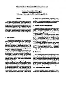
2. Data Collection The failure data is a set of failure time of the component. This failure time is always referred to Time Between Failure (TBF) of the component. TBF is measure from the time after a new component was installed until the time of next failure occurs. The measurement unit of TBF can be in operating hours, day and cycle. Figure 1 showed the graphical view of a set of TBF of the component in interval (t1, t2). x1
x2
x3
xi
t2
t1 Operating time
Figure 1 - Time between Failures (TBF) of the component
Proceedings of International Conference on Man-Machine Systems 2006 September 15-16 2006, Langkawi, Malaysia
The symbol of xi, shows the length of operating time (TBF) and i, is the number of failure time (number of data) at interval (t1, t2), which values of x are random. The length of operating time (TBF) depends on the type and how the component is designed and used.
F(ti) of each failure time can be determined using equation (1).
3. Identification the Best Fit Distribution and Its Parameters
While, the values of xi and yi axis can be determined using the formula tabulated in table 1.
Failure
Least-Squares Curve-Fitting (LSCF) technique is widely used for identifying the best fit distribution of failure time. The Maximum Likelihood Estimator (MLE) is used to identify the parameters of the distribution. The main objective in this paper is to propose a new approach by using LSCF and MLE in determination the best failure fit distribution and its parameters. The main advantage of the new approach is reduce the steps in determining the best fit distribution. Figure 2 showed the comparison in term of calculation steps between the traditional approach and the new approach proposed in this paper. Referring to figure 2, traditional approach generally has five steps in determining the best fit distribution and its parameters. In traditional approach, exponential, weibull, normal and lognormal distribution tests are used respectively to determine the best fit distribution. All these steps are under Least-Squares Curve-Fitting (LSCF) technique. In LSCF technique, the index of fit, r will be compared between exponential, weibull, normal and lognormal distribution tests. The higher value of r near to 1 will be selected as the best fit distribution. The last step (step number five) in the traditional approach is parameters estimation of best fit distribution using Maximum Likelihood Estimator (MLE) technique. However, in the new approach, only two steps are needed to identify the best failure fit distribution and its parameter. First step is to determine the shape parameter, β of weibull distribution using LSCF. The values of shape parameter, β shows the best distribution of failure time, as shown in figure 2; a new approach. Second step is estimating the distribution parameters depending on the shape parameter, β of weibull test using MLE. Following section present the calculation to determine the best fit distribution and its parameters for traditional approach and the new approach. 3.1 Traditional Approach Fit Distribution Test - Least-Squares Curve-Fitting (LSCF) Technique In the LSCF technique, a set of failure data will be arranged in a cumulative form. For example, if the failure time is assume to be a complete data (not censored), where the values are; 235, 259, 367, 214, 402, 115 and 98. The cumulative form of these failure times is 98, 115, 214, 235, 259, 367 and 402. Where n, is the total number of failure time and ti indicates the failure time and i, is the number of failure from minimum to maximum values. Then, three basic variables; cumulative function F(ti), xi and yi axis are determined for each distribution (exponential, weibull, normal and lognormal). The value of cumulative function,
F (t i ) =
(i − 0.3) ( n + 0.4)
(1)
Table 1- The value of xi and yi axis of the failure time Distribution
Step
xi
yi
Exponential Weibull
1 2
ti lnti
ln[1/(1 – F(ti)] lnln[1/(1 – F(ti)]
Normal Lognormal
3 4
ti ti
zi = Ф-1[F(ti)] = (ti –µ*)/σ* zi = Ф-1[F(ti)] = (lnti/σ *) (lnti/σ *)
Where, µ* and σ* is the initial value of mean and standard deviation of the sample, respectively. Each of these values can be determined using equation (2) and (3). n
µ* = ∑
ti n
∑ σ* =
i =1
i −1
n
(2)
t 2 − n( µ *) 2 n −1
(3) Finally, the index of fit, r is determined for each distribution test. The index of fit, r can be calculated using equation (4) [4]. The index of fit, r is compared between exponential, weibull, normal and lognormal distribution tests, which the higher value of, r will select as the best fit failure distribution. The parameters estimation is based on the distribution that chosen from the higher index of fit, r. n
r=
n
n
(∑ x i y i − ( ∑ x i ∑ y i ) / n) 2 i −1
n
i −1
n
i −1
n
n
i −1
i −1
(∑ x − (∑ x i ) / n)(∑ y 2 − (∑ y i ) 2 / n) 2
i −1
2
i −1
(4)
Parameter Estimation - Maximum Likelihood Estimator (MLE) technique Until the parameters are determined, the distribution is not completely specified [1]. Hence, the next step (step five) is to estimate the parameters of the distribution (highest index of fit, r) using Maximum Likelihood Estimator (MLE) technique. Each distribution has their particular parameters and it will be determined in different way. Table 2 shows the particular parameters of each distribution and their formula.
Proceedings of International Conference on Man-Machine Systems 2006 September 15-16 2006, Langkawi, Malaysia
Traditional Approach
A New Approach
A set of Data
A set of Data Least-Squares Curve-Fitting Test (Distribution test)
Least-Squares Curve-Fitting Test (Distribution test) Exponential test
Weibull test
Normal test
Weibull test
Lognormal test Determine initial shape parameter, β
Comparison the Index of fit, rx If, 0 < β < 1 (DFR) if re > rw ,rn and rl
Weibull
if rn > re ,rw and rl If, 1 < β < 3 (IFR)
if rw > re ,rn and rl
if rl > re ,rw and rn If, 3 ≤ β ≤ 4 (IFR)
If, β = 1 (CFR) Exponential
Parameter λ , failure rate
Weibull
Parameter θ , scale β , shape
Lognormal
Normal
Parameter µ , mean σ2 , variance
Normal
Exponential
Lognormal
Parameter µ , mean σ , standard deviation
Maximum Likelihood Estimator (MLE) Test
µ , mean σ2 , variance λ , failure rate
Maximum Likelihood Estimator (MLE) Test
Figure 2 – Comparison between traditional approach and a new approach in determination the best fit failure distribution and it parameters
θ , scale β , shape µ , mean σ , standard deviation
Proceedings of International Conference on Man-Machine Systems 2006 September 15-16 2006, Langkawi, Malaysia
3.2 Traditional Approach In the new approach it only used two steps for determining the best fit distribution and its parameters. Like the traditional approach, Least-Squares Curve-Fitting (LSCF) test is used in the process of identifying the best fit distribution. The basic idea in the new approach is determine the shape, β of weibull distribution. Theoretically, the shape parameter, β for weibull distribution presents different failure distribution depends on the value of, β (refer to figure 2 – a new approach) [1]. For example, if the value of shape parameter, β is between 3 ≤ β ≤ 4, the failure time follows the normal distribution trend. The cumulative form (equation (1)) and the values of xi and yi axis for weibull test (table 1) are used to determine shape parameter, β of weibull distribution. The value of β can be determined using equation (5) below;
Table 4 - The analysis results of Traditional Approach and A New Approach
∑ β=
3.4 Discussion The result from traditional approach shows the index of fit r, are tested for exponential, weibull, normal and lognormal distributions. The index of fit r, of exponential, weibull, normal and lognormal distribution test present the values of 0.8145, 0.9482, 0.9217, and 0.9106, respectively. The index of fit, r of weibull distribution shows higher value of 0.9482. Therefore, traditional approach concludes that the best fit failure distribution follows the weibull distribution. In the new approach result, the shape β, for weibull test is determined and the value of, β is 1.40. This result indicates that the best fit of the failure time (table 3) also follows the weibull distribution (refer to estimation of shape parameters, β in figure 2 – A new approach). The scale parameter, θ’ is calculated based on the table 2 formula, where, θ’ is 593.4. Both of traditional approach and the new approach shows a similar results, which the failure time (table 3) followed the weibull distribution. This result proved that the new approach proposed can be used as a practical technique in determining the best fit failure distribution.
n i =1
xi y i − x ∑i =1 y i
∑
n
n i =1
xi2 − n x
2
(5)
After the best distribution is determined depending on value of the shape parameter, β, the second step (final step) is use to determine the distribution parameters by using Maximum Likelihood Estimator (MLE) as shown in table 2. 3.3 Result Comparison – Numerical Example In this section, a set of failure times originally presented by Johnson (1964, p. 70) [3] was considered as a numerical example (table 3). The failure time is assumed as a complete data (not censored). The analysis results using both of traditional and a new approach are compared by using equations (1) to (5) and the calculation steps that have been discussed in the previous section. The analysis results between traditional approach and a new approach are summarized in table 4. Table 3 - Failure Times Originally Presented By [3] Failure time, t 112 213 250 484 500 572
Traditional approach Distributi Inde on test x of fit, r Exponent 0.814 ial 5 Weibull 0.948 2 Normal 0.921 7 Lognorm 0.910 al 6
A new approach Distributi on test Weibull
Shape paramet er, β 1.40
Shape parameter, β characteristic 1 < β < 3 = Failure time follow weibull distribution
4. Conclusion In this paper, a new approach to determine the best fit distribution is proposed. The basic idea in the new approach is determine the shape parameters, β of weibull distribution test. From the shape parameters, β, the best fit distribution of failure time can be predicted. Numerical example showed a similar result for both of traditional approach and the new approach. Simpler calculation steps to determine the best fit distribution is the main advantages by using a new approach compared to traditional approach that used require more calculation steps. This new approach can assist engineers to reduce the time analysis and the result is valid for maintenance strategies purposes.
Proceedings of International Conference on Man-Machine Systems 2006 September 15-16 2006, Langkawi, Malaysia
[4] Knezevic, J. 1993. Reliability, Maintainability and Supportability, The McRaw-Hill Companies, INC, London. [5] Maillart, L.M and Pollock, S.M. 1999. The effect of failure-distribution specification errors on maintenance cost, Proceedings Annual Reliability and Maintainability Symposium
References [1] Ebeling, C.E. 1997. Reliability and Maintainability Engineering, The McRaw-Hill Companies, INC, USA. [2] Jardine, A.K.S. 1973. Maintenance Replacement and Reliability, Pitman Publishing, Bath. [3] Johnson, L.G. 1964. Theory and Technique of Variation Research, Elsevier, Amsterdam.
Table 2 - Parameters and formula to estimate the parameters of each distribution
Distribution
Exponential
Parameter
Failure rate, λ’
Formula
λ'=
n = total number of
n
failure time
n
∑t
t = failure time
i
i −1
i = number of failure
Weibull
Shape parameter, β’
β=
∑
n
xi y i − x ∑i =1 y i n
i =1
∑
n i =1
xi2 − n x
2
1
Scale parameter, θ’
Normal
Variance, σ2’
Mean, µ’
1 n β ' θ ' = ∑ t iβ ' n i =1
σ2 =
( n − 1)σ * n
µ'= ∑
n
Lognormal
Mean, µ’
µ'= ∑ i =1
Standard deviation, σ’
σ '=
ti =x n
ln t i n
∑
n i =1
(ln t i − µ ' ) 2 n
time β = β’ n = total number of failure time i = number of failure time n = total number of failure time t = failure time i = number of failure time β’ = shape parameter n = total number of failure time σ* = variance from sample n = total number of failure time t = failure time i = number of failure time µ’= mean, µ* from sample n = total number of failure time t = failure time i = number of failure time n = total number of failure time t = failure time i = number of failure time µ’ = mean
Proceedings of International Conference on Man-Machine Systems 2006 September 15-16 2006, Langkawi, Malaysia