times, it is still useful to include the distance to each candidate host as a factor in ... traceroute can exceed the latency of a Web page access itself. ..... sured round-trip-time is the best metric to base server selection decisions upon, ..... Page 10 ...
IDMaps: A Global Internet Host Distance Estimation Service P. Francis S. Jamin C. Jin Y. Jin V. Paxson D. Raz Y. Shavitt L. Zhang Abstract There is an increasing need to quickly and efficiently learn network distances, in terms of metrics such as latency or bandwidth, between Internet hosts. For example, Internet content providers often place data and server mirrors throughout the Internet to improve access latency for clients, and it is necessary to direct clients to the closest mirrors based on some distance metric in order to realize the benefit of mirrors. We suggest a scalable Internet-wide architecture, called IDMaps, which measures and disseminates distance information on the global Internet. Higher-level services can collect such distance information to build a virtual distance map of the Internet and estimate the distance between any pair of IP addresses. We present our solutions to the measurement server placement and distance map construction problems in IDMaps. We show that IDMaps can indeed provide useful distance estimations to applications such as closest-mirror selection.1 Keywords: network service, distributed algorithms, scalability, modeling.
1 Introduction It is increasingly the case that a given service request from a client can be fulfilled by one of several Internet servers. Examples range from short-lived interactions such as a single Web page access to a Web server, to the long-term peering relationship between two news (NNTP) servers [3]. In all such interactions, all other things being equal, it is advantageous to access the “nearest” server with low latency or high bandwidth. Even when all other things are not equal, for instance, when different Web servers have different response times, it is still useful to include the distance to each candidate host as a factor in making a selection [4]. One method to obtain distance information is for the initiating host to measure it itself, using either unicast (ping, traceroute [5]) or multicast (expanding ring search [6]) tools. While these tools are easy to use, their utility is generally limited by their overhead. For instance, the latency of running a single traceroute can exceed the latency of a Web page access itself. More important still, a large number of hosts making independent and frequent measurements could have a severe impact on the Internet. Ideally, measurements made by one system (host or router) should be made available, with low overhead, to other hosts. A useful general service for the Internet should enable a host to quickly and efficiently learn the distance between any two hosts. To be widely useful, such a service should provide an answer with a delay and overhead less than the gain achieved by using the service. A simple protocol for such a service, SONAR, was discussed in the IETF as early as February 1996 [7], and in April 1997 as a more general service called HOPS (Host Proximity Service) [8]. Both of these efforts proposed lightweight client-server query/reply protocols similar to a DNS query/reply. The specifications also required each server to produce an answer in a very short time—preferably, though not necessarily, by using information already stored locally. As 1
Parts of this paper were previously published as [1] and [2].
1
stated, both services need some underlying measurement infrastructure to provide the distance measurements. In this paper, we propose a global architecture for Internet host distance estimation and distribution which we call “IDMaps” (Internet Distance Map Service). We intend to have IDMaps be the underlying service that provides the distance information used by SONAR/HOPS. We discuss the basic IDMaps architecture and show, through Internet experiments and simulation, that our approach can indeed provide useful distance information. In Section 2 we give an overview of our design goals, problem motivations, and the context of related works in which IDMaps is part of. In Section 3 we describe the basic IDMaps architecture: its components, distance measurement, and dissemination process. In Sections 3.2 and 3.3 we present several fundamental pertaining to IDMaps’ deployment. In Section 4 we present results from our performance evaluation of the IDMaps architecture.
2 Overview of IDMaps 2.1 IDMaps Goals A distance estimation service could be called upon to support a wide range of applications, from a client’s accessing a single page from a Web server once, to Network Time Protocol (NTP) servers establishing long term peering relationships with each another. Each application that can potentially find a distance estimation service useful will have its own set of requirements. IDMaps is not designed to satisfy all conceivable requirements for distance estimation service. For instance, we cannot hope for a general IDMaps service to provide near-instantaneous information about current delays and bandwidth seen between two Internet hosts, even though such information could be very useful to some applications. Rather, we have taken the opposite tack—we determined roughly the best service we may be able to provide given technology constraints and the need for global scalability of the service, and then considered whether there are applications for which this level of service would be useful. We now turn to a discussion of the resulting goals.
Separation of Functions: We envision IDMaps as an underlying measurement infrastructure to support a distance information query/reply service such as SONAR. The full separation of IDMaps and the query/reply service is necessary because the different functionalities place different constraints on the two systems. The requirements for IDMaps are relative accuracy of distance measurements with low measurement overheads, while the requirements for the query/reply service are low query latency, high aggregate query throughput, and reasonable storage requirements. By decoupling the different functionalities, we can streamline the design of IDMaps to perform measurements with low overheads and allow the query/reply service to make flexible uses of the measured distances. IDMaps’ design must be robust to provide continued, though maybe less accurate, services even in the face of component failures. Furthermore, given the continued growth of the Internet, the system must scale effortlessly, utilizing new IDMaps servers whenever and wherever they appear. This calls for a design that allows IDMaps servers to be added or removed by any authorized party, at any time, at any location. IDMaps servers must be autonomous entities which monitor and measure their changing environments with minimal human intervention.
2
Distance Metrics: Our goal is to provide distance information in terms of latency (e.g., round-trip delay) and, where possible, bandwidth. Latency is the easiest sort of information to provide, and luckily the most generally useful. There are two reasons latency information is easy to provide. First, it is easy to measure. A small number of packets can produce a good coarse-grain estimate. Second, two different paths may have the same latency such that while our probe packets may not travel the same path as the path actually taken by the users’ data packet, the reported latency would still be useful. Bandwidth is also clearly important for many applications, but compared to latency, bandwidth is more difficult to provide. It is more expensive to measure, and it is also more sensitive to the exact path—a single low-bandwidth link dictates the bandwidth for the whole path. It may also be that there is a rough correspondence between latency and bandwidth—that is, the lower the latency between two hosts, the higher the bandwidth is likely to be, thus allowing applications that need high-bandwidth to minimize latency as a first approximation.
Accuracy of the Distance Information: We believe highly accurate distance estimates (say, within 5% of the distance measured by the end-host itself) are impossible to achieve efficiently for a large scale Internet service. While we may be able to achieve this level of accuracy for each path measured, an estimate based on triangulation of such the measurements will see an accumulation of the error terms. Instead, our goal is to obtain accuracy within a factor of 2 with very high probability and often better than that. We expect this level of accuracy to be adequate for SONAR and HOPS servers. It would, for instance, allow an application to select the closest Web server among ones that are reported to be 20 ms, 100 ms, and 500 ms away. The (reported) 20 ms server, which might actually be as far as 40 ms, would still be better than the (reported) 100 ms server, which might be as close as 50 ms. Being able to distinguish systems that are very close, very far, or somewhere in between is useful for a wide range of applications. For those that require more accurate measurements, they may at least use this coarse-grained information as a hint to server selection.
Timeliness of the Distance Information: We must consider two kinds of distance information— load sensitive and “raw” (distances obtained assuming no load on the network, which generally can be approximated by saving the minimum of a number of measurements). In the interest of scalability, we plan to provide the raw distance information with an update frequency on the order of days, or if necessary, hours. In other words, the distance information will not reflect transient network conditions, and will only adjust to “permanent” topology changes. Instantaneous or near-instantaneous (within 15 or 20 seconds) load information is both impossible to distribute globally and of diminishing importance to future applications: as the Internet moves to higher and higher speed, the propagation delay will become the dominant factor in distance measurements.2
Scope of the Distance Information: We assume that the distance information applies only to the “public” portion of the Internet—the backbone networks, BGP information, and possibly the public side of firewalls and border routers of private networks. Even if distance information of private networks were obtainable, it may be desirable not to include it for scalability reasons. This is not to suggest that distance information inside private networks is not important. We believe the architecture presented in this proposal can be replicated within a private network, but otherwise do not address distance measurement within private networks. 2
While propagation delay is lower bounded by geographic distance, it is determined by topological distance. Given the dynamic nature of Internet topology, changes to topological distances can be scalably tracked only by an automatic system such as IDMaps.
3
2.2 Alternative Architectures and Related Works The primary motivation of IDMaps is to provide an estimate of the distance between any two valid IP addresses on the Internet. It is important to discuss this motivation because it significantly differentiates IDMaps from other services that also provide distance information, e.g., the SPAND, Remos, IPMA, NIMI, and MINC projects [9, 10, 11, 12, 13]. These projects serve various purposes, such as general Internet characterization, maintenance, fault-isolation, and end-system distance estimation; IDMaps, on the other hand, aspires to be a public infrastructure that provides distance information between any two arbitrary points on the Internet, where the querying entity is not one of the two end points. An alternative to providing distance information between arbitrary pairs of hosts on the Internet would be a localized service that provides only distance information between hosts close to a distance server and remote hosts on the Internet. Such a service is simpler to provide because the amount of information each distance server has to work with scales at the order of number of possible destinations ( ), instead of the order of IDMaps’—all possible pairs of Internet destinations. SONAR and SPAND propose this type of service. Localized distance service, however, works well when only a few networks conduct distance measurements. With the increase in applications that require distance information, such as peer-to-peer file sharing and client-hosted multiplayer gaming, the aggregated load of localized distance service will scale . The amount of measurement traffic under IDMaps will likely be much smaller than the on the order of order because of the global sharing of distance information and as a result of our application of graph compression techniques such as -spanners (see Sections 3.3.1 and 4.4). The administrative cost of setting up and maintaining IDMaps service is also fixed. It has been argued in [9] that passive measurement has an advantage over active measurement in not sending additional traffic and perturbing actual Internet traffic. Although the non-intrusive nature of passive measurement is very appealing, passive measurement has its limitations:
�� ��
��
�
1. Passive monitoring can only measure the regions of the Internet that application traffic has traversed. A service that relies solely on passive monitoring may not be able to discover the distance to unknown networks/hosts. For example, a client trying to choose the nearest among multiple copies (or mirrors) of a Web server will require distance information between the client and all such mirrors. A passive monitoring system can only provide distance information to mirrors that have been previously accessed, either by the client or others within its proximity. 2. Passive monitoring has only one view of the Internet because only end-to-end path data is collected. When Internet topology changes, for example, due to an upgrade of some provider’s backbone network, passive monitoring may be forced to re-collect most if not all of its distance information. Although IDMaps also uses end-to-end measurements, the end-to-end distances in IDMaps are collected from multiple, intermediate, points on the Internet, this allows the distance database to locate any topological change and update only those actually effected. 3. The responsibility of deploying passive monitoring based distance service rests on the administrator of each individual network and requires certain expertise and resources. With IDMaps, network administrators only need to install a querying system, which can be standardized similar to DNS (Domain Name System). 4. Finally, passive measurement typically requires some kind of monitoring or snooping of network traffic, which may raise privacy and security concerns. Another alternative to providing distance information on the Internet is by charting the physical connectivities between nodes (hosts and routers) on the Internet and computing a spanning tree on the resulting connectivity map. Distances between pairs of nodes can then be estimated by their distances on the spanning tree. We call this alternative the hop-by-hop approach. The projects described in [14, 15, 16, 17]
4
provide snapshots of the Internet topology at the hop-by-hop level. This approach largely relies on sending ICMP (Internet Control Message Protocol) packets to chart the Internet. To minimize perturbation to the network, each snapshot of the topology is usually taken over a period of weeks, hence the result does not adapt well to topological changes. More seriously however, due to the recent increased in security awareness on the Internet, such measurement probes are often mistaken for intrusion attempts. To motivate the service provided by IDMaps, in this paper we present some results on how it can be used in the nearest mirror selection problem. The problem of mirror selection and mirror ranking has been studied extensively in the literature, for example by the authors of [18, 19, 20, 21, 22, 23, 24, 25, 26, 9]. Previous works on mirror selection can be classified into three categories: network-layer server selection, application-layer server selection, and measurement-based server selection. In network-layer server selection, the closest server in terms of number of hops (AS hops or router hops) [27] or in terms of network latency [20] is selected. In application-layer server selection, some application performance metrics (e.g., server load and available bandwidth) were taken into account while selecting a server [18, 9]. In measurement-based server selection, set of measurements (e.g., actual download of data objects from different mirrors) are conducted to rank different mirrors [23]. In [23], the authors measured nine clients scattered throughout the United States retrieving documents from fourty-seven Web servers, which mirrored three different Web sites. They presented findings that revealed good stability of mirror rankings according to download time. In [28], the authors presented a server selection techniques that can be employed by clients on end hosts. The technique itself involves periodic measurements from clients to all of the mirrors. Finally, as already mentioned, the authors of [9] proposed a server selection scheme based on shared passive end-to-end performance measurements collected from clients in the same network. The effectiveness of client-side mirror selection and provider-side mirror selection were studied in [21] and [29, 26] respectively. The authors of [18, 21] studied different distance metrics and concluded that measured round-trip-time is the best metric to base server selection decisions upon, for different data object sizes. We emphasize that the nearest mirror selection problem is used only as a motivational example in this paper. We do not intend to study nearest mirror selection problem exhaustively in this paper.
3 IDMaps Architecture This section outlines the IDMaps architecture. Specifically, we address the following three questions: 1. What form does the distance information take? 2. What are IDMaps’ components? 3. How should the distance information be disseminated?
3.1 Various Forms of Distance Information The conceptually simplest and most accurate form of distance information IDMaps can measure consists of distances between any pair of globally reachable IP addresses 3 (as shown in Figure 1). The distance from one IP address to another is then determined by simply indexing the list to the appropriate entry (using �� �� , a hashing algorithm) and reading the number. The large scale of this information (on the order of � where , number of hosts, could be hundreds of millions) makes this simple form of distance infeasible, as does the task of finding all such hosts in an ever-changing Internet in the first place. The next simplest would be to measure the distances from every globally reachable Address Prefix (AP) on the Internet to every other (Figure 1). An AP is a consecutive address range of IP addresses within
�
3
Understanding here that different IP addresses may be reachable at different times, given technologies like NAT and dial-up Internet access.
5
Host in BGP prefix in AS (Autonomous System) Host A2 + P’ cost H2 cost
A = number of ASs P’ = number of BGP prefixes
H = number of Hosts
(A
-
:
Waxman. .-Under the Waxman the probability that an edge is formed between �� �� � .- � - nodes and is � ����model, � � � # , where � � is the Euclidean distance between and and is the given by maximum possible distance between any two nodes on the generated network. A random .- � number between�� � . We use
0 and 1 is generated. The edge is added if this number is smaller than the computed � � � � , which give us a mean node degree of around 2.2. Finally, a spanning tree is computed, and adding edges where necessary, such that the final network is a connected graph.
: 6
:
:
:
6
6
Tiers. Tiers places the given nodes on the � ! � plane ensuring that nodes are not within a radius of
� �� � of each other. Edges are added by first computing a minimum spanning tree connecting the nodes. Each node is then connected to as many other nodes as specified by its node degree. In selecting a node’s neighbors, the ones closest to the node that have not yet met their node degrees are selected first. The connectivity degree of each node is randomly distributed with a maximum node degree (WAN redundancy, in Tiers parlance) of . Fig. 10 shows the distribution of the resulting node degree on our 1,000 node � � . network for �
E
E 6
Inet. Motivated by the recent findings on the power-law relationship between node (Autonomous System) vertex degree and the frequency distribution of the vertex degrees [52], we designed a topology generator to produce graphs with such power-law relationship. We call our generator Inet and described it more fully � � nodes with the highest vertex degrees into a full-mesh. Then in [2].8 Briefly, we first connect the � to simulate the geographically dispersed nature observed of large ISPs’ networks, we expand the most connected � nodes into networks with � randomly placed nodes each. In this paper, we use � � � for � � � � � � � , and � � � � � � , � � � in all cases. for For each of the three models, we generate thirty-one networks with 1,000 nodes and thirty-one networks with 4,200 nodes each, for a total of 186 random topologies. Fig. 10 shows the distribution of node degree of three generated topologies, one each from the three models. Table 2 lists the diameter and the maximum node degree of the three networks, and Figs. 11 and 12 show the distribution of hop counts and end-to-end distance between all node pairs in the three networks respectively. In Fig. 11 (12) the hop counts (e2e distances) are normalized by the diameter of the respective network.
6
6
8
6
6
1
Normalized E2E Distance
6
6
Our Inet topology generator is available for download from http://topology.eecs.umich.edu/inet/.
17
Model Waxman Tiers Inet
Hop Count 21 35 18
E2E Distance 77,655 14,635 78,379
Max Node Degree 8 20 24
Table 2: Network diameter and max node degree
4.2 Simulating IDMaps Infrastructure Once a network is generated, we “build” an IDMaps infrastructure on it. In this section, we describe how the various Tracer placement and distance map computation algorithms and heuristics are implemented.
Tracer Placement. In Section 3.2, we described two graph-theoretic approaches to Tracer placement and three heuristics. We implement the graph-theoretic approaches, we compute Tracer placement using the algorithms described. To implement Stub-AS Tracer placement, given Tracers, we pick nodes with the lowest degrees of connectivity to host Tracers. Conversely, for Transit-AS placement, we pick nodes with the highest degrees of connectivity. We implement Mixed Tracer placement by giving equal probability to all nodes on the generated network to host a Tracer.
Distance Map Computation. A distance map consists of two parts: Tracer-Tracer VLs and TracerAP VLs. Each Tracer advertises the VLs it traces. We do not simulate VL tracing and advertisement or AP discovery in this study, and we only simulate a single IDMaps Client. Since IDMaps Clients operate independently, the use of a single IDMaps Client has no loss of generality. The simulated IDMaps client has a full list of Tracers and their locations. The Tracer-Tracer part of the distance map is computed either assuming a full-mesh among all Tracers, or by executing the original -spanner algorithm shown in Fig. 7. Each AP (node) can be traced by one or more Tracers. When each AP is traced by a single Tracer, the Tracer closest to an AP is assigned to trace to the AP. If an AP is to be traced by more than one Tracer, Tracers are assigned to the AP in order of increasing distance. In our simulations, we assume all edges are bidirectional, and paths have symmetric and fixed costs. We study the effect of measurement error and stability on IDMaps’ performance in a related work [53]. Once a distance map is built, the distance between two APs, � and is estimated by summing up the �� �� , the distance from to its nearest Tracer distance from � to its nearest Tracer �� �� �� �� , and the distance between and . When a full-mesh is computed between Tracers, the to distance is exactly the length of the shortest path between them on the underlying network. Otherwise, they are computed from the -spanner. If � and have multiple Tracers tracing to them, the distance between � and is the shortest among all combinations of Tracer-AP VLs and Tracer-Tracer VLs for the Tracers and APs involved.
�
�
4.3 Performance Metric Computation Ultimately, IDMaps will be evaluated by how useful its distance information is to applications. In this paper, we evaluate the performance of IDMaps using nearest mirror selection as a prototypical application and adopt an application-level performance metric, ���� , which measures how often the determination of the closest mirror to a client, using the information provided by IDMaps, results in a correct answer, i.e., the mirror the client would have been redirected based on a shortest path tree constructed from the underlying physical topology. Incidentally, the localized distance measurement service (see Section 2.2) such as provided by [9, 18] in effect constructs a shortest-path tree from each client (or stub network) to all mirrors.
���� thus can be considered as comparing the performance of IDMaps against the localized services in the
18
Topology Waxman Tiers Inet
Placement Stub-AS Transit-AS Mixed Min -center � -HST
10 20 40 100
T-T Map full-mesh 2-spanner 10-spanner
T/AP 1 2 3
Table 3: Simulation Parameters best case scenario for the localized services, i.e., the distances from the clients to all mirrors are known a priori and were obtained at no cost. Performance comparison between localized services and IDMaps in the common case must take into account the shortcomings of localized services (see Section 2.2), chief among which is the time lag in obtaining distance to “uncharted” parts of the Internet due to the “on-demand” nature of the service, and the additional cost of collecting distance information due to the lack of information sharing between clients and the cost of maintaining each instance of the localized service. Considering, however, that the goal of IDMaps is not to provide precise estimates of distances between hosts on the Internet, but rather estimates of relative distances between a source (e.g. a client) and a set of potential destinations (e.g. server mirrors), we adopt a lax version of this measure in this paper, as follows. In each simulation experiment, we first place � (from 3 to 24) server mirrors in our simulated network. We place the mirrors such that the distance between any two of them is at least � � the diameter of the network. We consider all the other nodes on the network as clients to the server. We then compute for each client the closest server according to the distance map obtained from IDMaps and the closest server according to the actual topology. For a given � -mirror placement, we compute ��� as the percentage of correct IDMaps’ answers over total number of clients. Considering that on the Internet, a client served by a server 15 ms away would probably not experience a perceptible difference from being served by a server 35 ms away, or that a server 200 ms away will not appear much closer than one 150 ms away, we consider IDMaps’ server selection correct as long as the distance between a client and the closest server determined by IDMaps is within a factor of � times the � ). distance between the client and the actual closest server (in this paper, we use � We repeat this procedure for 1,000 different � -mirror placements, obtaining 1,000 ���� values in each experiment. In the next section, we present our simulation results by plotting the complementary distribution function9 of these ���� values. �
�6
4.4 Simulation Results Table 3 summarizes the parameters of our simulations. The heading of each column specifies the name of the parameter, and the various values tried are listed in the respective column. The column labeled “Topology” lists the three models we use to generate random topologies. The “Placement” column lists the Tracer placement algorithms and heuristics. The “ ” columns lists the number of Tracers we use on 1000-node networks. The “T-T Map” column lists the methods used to compute the Tracer-Tracer part of the distance map. The “T/AP” column lists the number of Tracers tracing to an AP. We experimented with almost all of the 540 possible combinations of the parameters on 1,000 node networks and several of them on 4,200 node networks. In addition, we also examined the case of having more mirrors for a few representative simulation scenarios. 9
The complementary distribution function, variable .
��
�# ��� � � � #� � , where � �� � is the cumulative distribution function of the random
19
0.6 0.4 Transit AS k-HST Random Selection
0.2 0 40
50
60
70
80
90
100
1 0.8 0.6 0.4 Transit AS k-HST Random Selection
0.2 0 40
50
Percentage of Correct Answers
60
70
80
90
100
Complementary Distribution Function
0.8
Complementary Distribution Function
Complementary Distribution Function
1
1 0.8 0.6 0.4 Transit AS k-HST Random Selection
0.2 0 40
50
Percentage of Correct Answers
a. Inet
60
70
80
90
100
Percentage of Correct Answers
b. Waxman
c. Tiers
Figure 13: 3-Mirror selection on 1,000-node network with 10 Tracers.
0.8
0.6
0.4
0.2 Transit AS k-HST Random Selection 0
1
Complementary Distribution Function
1
Complementary Distribution Function
Complementary Distribution Function
1
0.8
0.6
0.4
0.2 Transit AS k-HST Random Selection 0
0
20
40
60
80
100
Percentage of Correct Answers
a. Inet
0.8
0.6
0.4
0.2 Transit AS k-HST Random Selection 0
0
20
40
60
Percentage of Correct Answers
b. Waxman
80
100
0
20
40
60
80
Percentage of Correct Answers
c. Tiers
Figure 14: 24-Mirror selection on 1,000-node network with 10 Tracers. The major results of our study are: 1. Mirror selection using IDMaps gives noticeable improvement over random selection. 2. Network topology can affect IDMaps’ performance. 3. Tracer placement heuristics that do not rely on knowing the network topology can perform as well as or better than algorithms that require a priori knowledge of the topology. 4. Adding more Tracers (over a 2% threshold) gives diminishing return. 5. Number of Tracer-Tracer VLs required for good performance can be on the order of with a small constant. 6. Increasing the number of Tracers tracing to each AP improves IDMaps’ performance with diminishing return. These results apply to both the 1,000-node and 4,200-node networks. We present simulation data substantiating each of the above results in the following subsections. Due to space constraints, we are not able to include data confirming some of these results on the Internet [54].
4.4.1 Mirror Selection Results presented in this subsection are obtained from simulations on 1,000-node randomly generated topologies. In all cases, 3 mirrors are manually placed on the network, the number of Tracers deployed is 10 (1% of nodes), the distance maps are built by computing full-meshes between the Tracers, with only a single Tracer tracing to each AP. We compare the results of random selection against selection using the distance map generated by IDMaps. The metric of comparison is ���� . Each line in Fig. 13 shows the complementary distribution function of 1,000 ���� values as explained in the previous section. Each line is the average of 31 simulations
20
100
using different random topologies, the error bars show the 95% confidence interval. For example, the line labeled “Transit-AS” in Fig. 13a shows that on an Inet-generated topology, when mirrors are selected based on the distance map computed from Tracers placed by the Transit-AS heuristic, the probability that at least 80% of all clients will be directed to the “correct” mirror is 100% (recall our definition of correctness from the previous section); however, the probability that up to 98% of all clients will be directed to the correct mirror is only 85%. We start the x-axis of the figure at 40% to increase legibility. The line labeled “ � -HST” is the result when the � -HST algorithm is used to place Tracers. The � -HST algorithm requires knowledge of the topology (see Section 3.2.1). The line labeled “Random Selection” is the result when mirrors are randomly selected without using a distance map. As expected, it performs well for less than 40% correctness and the performance deteriorates beyond 60% correctness. Mirror selection using distance maps outperforms random selection regardless of the Tracer placement algorithm. We include only the best and worst performing Tracer placement algorithms in Figs. 13 for legibility of the graphs. The relative performance of the various placement algorithms is presented in Section 4.4.3. Fig. 14 shows results from simulations with 24 mirrors. Qualitatively, these results agree with our conclusion that mirror selection using distance maps ourperforms random selection.
4.4.2 Effect of Topology Figs. 13b and 13c show the results of running the same set of simulations as in the previous section, but on topologies generated from the Waxman and Tiers models respectively. Again, the error bars on each figure shows the 95% confidence interval computed from 31 randomly seeded topologies. While mirror selection using a distance map provides better performance than random selection in all cases, performance on the Tiers generated topology exhibit a qualitatively different behavior than those in the other two topologies. For example, the Transit-AS heuristic gives better IDMaps performance than the � -HST algorithm on topologies generated from the Inet and Waxman models, but not so in the topology generated from Tiers. We offer a hypothesis for the relatively poor performance of random mirror selection on Tiers topology. Fig. 12 shows that almost all the end-to-end distances in Inet generated network fall between 20% and 60% of the network diameter. When we randomly pick two distances from this network, it is highly likely that they will fall within this range. Consequently, one distance will be no more than 3 times longer than the other. So given our definition of the performance metric, even the random selection can give acceptable performance. As can be seen by comparing Fig. 13b against Figs. 13a and 13c, this is more evident in the network generated from the Waxman model, where the distances fall between 30% and 70% of the network diameter. However, the distance distribution for the Tiers topology is much more dispersed, and the range is between 10% and 70% of the diameter. It is much harder for two randomly picked distances to be close within a factor 3. This is corroborated by the poor results “Random Selection” returns. We note again that despite the significant differences in the three models, IDMaps is able to provide noticeable improvements in mirror selection in all three cases.
4.4.3 Performance of Placement Algorithms To compare the relative performance of the various Tracer placement algorithms and heuristics, we repeat the same simulations as in the previous two subsections, once for each placement algorithm. Then using the complementary distribution function of the ���� values obtained from running the Mixed placement algorithm as the baseline, we compute the improvement of each placement algorithm relative to Mixed placement. The results are presented in Figs. 15a, 15b, and 15c for networks generated using the Inet, Waxman, and Tiers models respectively. There is no clear winning placement algorithm across all topologies, but the minimum -center algorithm and Transit placement consistently performed well in all three topologies. In general, the simple heuristics can often perform as well as the graph theoretic placement
3
21
25
50 Transit AS Min-K Stub AS k-HST
250 Transit AS Min-K Stub AS k-HST
15 10 5 0 -5 -10
30 20 10 0
-20
-20 40
50
60
70
80
90
100
150
100
50
0
-10
-15
Transit AS Min-K Stub AS k-HST
200 Percentage of Improvement
40 Percentage of Improvement
Percentage of Improvement
20
-50 40
50
Percentage of Correct Answer
60
70
80
90
100
40
Percentage of Correct Answer
a. Inet
50
60
70
80
90
100
Percentage of Correct Answer
b. Waxman
c. Tiers
Figure 15: Improvement of placement algorithms over the “Mixed” algorithm on 1,000-node network, 10 Tracers. 1
Complementary Distribution Function
Complementary Distribution Function
1
0.8
0.6
0.4
10 Tracers 20 Tracers 40 Tracers 80 Tracers 100 Tracers
0.2
0
0.8
0.6
0.4
10 Tracers 35 Tracers 70 Tracers 140 Tracers 350 Tracers
0.2
0 40
50
60 70 80 Percentage of Correct Answers
90
100
80
a. 1,000-node Tiers network
85
90 95 Percentage of Correct Answers
100
b. 4,200-node Inet network
Figure 16: Mirror selection using IDMaps with varying number of Tracers. strategies. In [54] we also present results of applying the graph theoretic placement algorithms on distance maps computed from the Transit-AS heuristics.
4.4.4 Having More Tracers In this subsection, we study the effect of increasing the number of Tracers on IDMaps’ performance. Fig. 16a shows the results of running the Transit-AS placement algorithm on a 1,000-node network generated using the Tiers model. Increasing the number of Tracers from 10 to 20 improves performance perceptibly, with diminishing improvements for further increases. Comparing Fig. 16a against Fig. 13c from Section 4.4.2 we see that increasing the number of Tracers from 10 to 20 makes the performance IDMaps using the Transit-AS placement algorithm comparable to that using the � -HST algorithm with 10 Tracers. Fig. 16b shows the results of running the Transit-AS placement algorithm on a 4,200-node network generated using the Inet model. Again, we see a perceptible improvement in IDMaps performance when the number of Tracers increases from 10 to 35, with diminishing improvements for further increases. Also of significance is that having only .2% of all nodes serving as Tracers already provides correct answer 90% of the time with very high probability. Overall, it is clear that we do not necessarily need a large scale IDMaps deployment to realize an improvement in the current metric of interest, ���� .
22
40 2 Tracers per AP 3 Tracers per AP
35 0.8 Percentage of Improvement
Complementary Distribution Function
1
0.6
0.4
30 25 20 15 10
0.2 Full Mesh 2-spanner 10-spanner
5
0
0 40
50
60
70
80
90
100
80
85
Percentage of Correct Answers
Figure 17: Effect of � -spanner on 1,000-node I net network with 100 Tracers. Model Placement Stub Mixed Transit Min -center
2-spanner 628 520 434 402
90
95
100
Percentage of Correct Answers
Inet 10-spanner 198 200 198 198
Figure 18: Mirror selection on 1,000-node Waxman network with 2 and 3 Tracers / AP. Waxman 2-spanner 10-spanner 654 198 466 198 386 202 434 196
Tiers 2-spanner 10-spanner 268 202 264 200 262 198 266 202
Table 4: Number of VLs in � -spanners of 100 Tracers . 4.4.5 Distance Map Reduction In all the simulations reported so far, the distance maps are built by computing full-mesh Tracer-Tracer VLs. Figure 17 shows the results of running the Transit-AS algorithm to place 100 Tracers on a 1,000node network generated using the Inet model, with Tracer-Tracer VLs computed as a full-mesh and as -spanners. For � , there is no perceptible difference in performance; for � � , the performance is worse. Qualitatively similar results are observed for topologies generated by the Waxman and Tiers models, with worse performance for � � in the Tiers case. Using a -spanner in place of a full-mesh can significantly reduce the number of Tracer-Tracer VLs that must be traced, advertised, and stored. Table 4 shows that for all the topologies we experimented with, the number of VLs used by both 2- and 10-spanners are on the order of with a small constant multiplier. In � � � is 4,950 edges. contrast, the number of VLs required to maintain a full-mesh for
�
� 6
�
� 6
�/6
6
4.4.6 Multiple Tracers per AP In all our simulations so far we have assumed that only a single Tracer traces each AP. We showed in Section 3.3.2 (Fig. 8) that in some cases having more than one Tracer tracing an AP may result in better distance estimates. We now present some performance results from scenarios in which there are 2 or 3 Tracers tracing each AP. On 1000-node networks, we place 100 Tracers using the Transit-AS algorithm, and compute a full-mesh for Tracer-Tracer VLs. Using the performance of IDMaps where only one Tracer traces each AP as the baseline, we compute the percentage improvement of increasing the number of Tracers per AP. Fig. 18 shows that on a 1000-node network generated using the Waxman model, compared to having only one Tracer per AP, the probability of having at least 98% correct answer is increased by 17% when each AP is traced by 2 Tracers, and is increased by 25% when each AP is traced by 3 Tracers. We only
23
consider up to 3 Tracers per AP since currently 85% of ASs in the Internet have degree of connectivity of at most 3 [52].
5 Conclusion It has become increasingly evident that some kind of distance map service is necessary for distributed applications in the Internet. However, the question of how to build such a distance map remains largely unexplored. In this paper, we propose a global distance measurement infrastructure called IDMaps and tackle the question of how it can be placed on the Internet to collect distance information. In the context of closest server selection for clients, we showed that, significant improvement over random selection can be achieved using placement heuristics that do not require the full topological knowledge. In addition, we showed that the IDMaps overhead can be minimized by grouping Internet addresses into APs to reduce the number of measurements, the number of Tracers required to provide useful distance estimations is rather small, and applying -spanners to the Tracer-Tracer VLs can result in linear measurement overhead with respect to the number of Tracers. Overall, this study has provided positive results to demonstrate that a useful Internet distance map service can indeed be built scalably.
�
References [1] P. Francis et al., “An Architecture for a Global Internet Host Distance Estimation Service,” Proc. of IEEE INFOCOM 1999, March 1999. [2] S. Jamin et al., “On the Placement of Internet Instrumentation,” Proc. of IEEE INFOCOM 2000, March 2000. [3] B. Kantor and P. Lapsley, “Network news transfer protocol: A proposed standard for the stream-based transmission of news,” RFC 977, Internet Engineering Task Force, Feb. 1986. [4] S. Bhattacharjee et al., “Application-Layer Anycasting,” Proc. of IEEE INFOCOM ’97, Apr. 1997. [5] W. Stevens, TCP/IP Illustrated, Volume 1: The Protocols, Addison-Wesley, 1994. [6] S.E. Deering and D.R. Cheriton, “Multicast Routing in Internetworks and Extended LANs,” ACM Transactions on Computer Systems, vol. 8, no. 2, pp. 85–110, May 1990. [7] K. Moore, J. Cox, and S. Green, “Sonar - a network proximity service,” http://www.netlib.org/utk/projects/sonar/, Feb. 1996.
Internet-Draft, url:
[8] P. Francis, “Host proximity service (hops),” Preprint, Aug. 1998. [9] M. Stemm, R. Katz, and S. Seshan, “A Network Measurement Architecture for Adaptive Applications,” Proc. of IEEE INFOCOM ’00, pp. 2C–3, Mar. 2000. [10] N. Miller and P. Steenkiste, “Collecting Network Status Information for Network-Aware Applications,” Mar. 2000. [11] C. Labovitz et al., “Internet performance measurement and analysis project,” http://www.merit.edu/ipma/, 1998.
url:
[12] V. Paxson, J. Mahdavi, A. Adams, and M. Mathis, “An Architecture for Large-Scale Internet Measurement,” IEEE Communications Magazine, vol. 36, no. 8, pp. 48–54, August 1998. [13] A. Adams et al., “The Use of End-to-End Multicast Measurements for Characterizing Internal Network Behavior,” IEEE Communications Magazine, pp. 152–158, May 2000.
24
[14] R. Govindan and H. Tangmunarunkit, “Heuristics for Internet Map Discovery,” Proc. of IEEE INFOCOM 2000, 2000. [15] R. Siamwalla, R. Sharma, and S. Keshav, “Discovering Internet Topology,” Unpublished manuscript. [16] K. C. Claffy and D. McRobb, “Measurement and Visualization of Internet Connectivity and Performance,” http://www.caida.org/Tools/Skitter/. [17] Hal Burch and Bill Cheswick, “Mapping the Internet,” IEEE Computer, vol. 32, no. 4, pp. 97–98, April 1999. [18] Robert L. Carter and Mark E. Crovella, “Server Selection using Dynamic Path Characterization in Wide-Area Networks,” Proc. of IEEE INFOCOM ’97, April 1997. [19] Robert L. Carter and Mark E. Crovella, “Dynamic Server Selection using Bandwidth Probing in Wide-Area Networks,” Tech. Rep. BU-CS-96-007, Boston University, March 1996. [20] Mark E. Crovella and Robert L. Carter, “Dynamic Server Selection in the Internet,” Proc. of IEEE Workshop on the Architecture and Implementation of High Performance Communication Subsystems’95, June 1995. [21] Sandra G. Dykes, Clinton L. Jeffery, and Kay A. Robbins, “An Empirical Evaluation of Client-Side Server Selection Algorithms,” Proc. of IEEE INFOCOM ’2000, 2000. [22] James D. Guyton and Michael F. Schwartz, “Locating Nearby Copies of Replicated Internet Servers,” Proc. of ACM SIGCOMM ’95, pp. 288–298, 1995. [23] A. Myers, P. Dinda, and H. Zhang, ““Performance Characteristics of Mirror Servers on the Internet”,” Proc. of IEEE INFOCOM ’99, Mar. 1999. [24] Katia Obraczka and Fabio Silva, “Looking at Network Latency for Server Proximity,” Tech. Rep. USC-CS-99-714, University of Southern California, 1999. [25] M. Sayal, Y. Breibart, P. Scheuermann, and R. Vingralek, “Selection Algorithms for Replicated Web Servers,” Performance Evaluation Review, vol. 26, no. 3, pp. 44–50, Dec 1998. [26] Anees Shaikh, Renu Tewari, and Mukesh Agrawal, “On the Effectiveness of DNS-based Server Selection,” Proc. of IEEE INFOCOM ’2001, 2001. [27] P.R. McManus, “A passive system for server selection within mirrored resource environments using as path length heuristics,” http://proximate.appliedtheory.com/, Jun. 1999. [28] Zongming Fei, Samrat Bhattacharjee, Ellen W. Zegura, and Mostafa Ammar, “A novel server selection technique for improving the response time of a replicated service,” Proc. of IEEE INFOCOM, 1998. [29] V. Cardellini, M. Colajanni, and P.S. Yu, “Dynamic Load Balancing on Web Server Systems,” IEEE Internet Computing, pp. 28–39, May-June 1999. [30] T. Bates, “The CIDR Report,” url: http://www.employees.org/˜tbates/cidr-report.html, June 1998. [31] Y. Rekhter and T. Li, “A border gateway protocol 4 (bgp-4),” RFC 1771, Internet Engineering Task Force, Mar. 1995. [32] R. Govindan and H. Tangmunarunkit, ““Heuristics for Internet Map Discovery”,” Proc. of IEEE INFOCOM 2000, pp. 3C–2, Mar. 2000. [33] T.H. Cormen, C.E. Leiserson, and R.L. Rivest, Introduction to Algorithms, Cambridge, MA: MIT Press, 1990.
25
[34] S. Hotz, “Routing Information Organization to Support Scalable Interdomain Routing with Heterogenous Path Requirements,” Tech. Rep. Ph.D. Thesis, Univ. of Southern California, CS Dept., 1994. [35] J.D. Guyton and M.F. Schwartz, “Locating Nearby Copies of Replicated Internet Servers,” Proceedings of ACM SIGCOMM, August 1995. [36] S. Savage et al., “The End-to-End Effects of Internet Path Selection,” Proc. of ACM SIGCOMM ’99, Sep. 1999. [37] V. Paxson, “End-to-End Routing Behavior in the Internet,” Proc. of ACM SIGCOMM ’96, pp. 25–38, Aug. 1996. [38] Merit Networks, “Npd (network probe daemon) project,” URL: http://www.merit.edu/ipma/npd/, 1996. [39] MirrorNet, “Multiple traceroute gateway,” URL: http://www.tracert.com, 1999. [40] Y. Bartal, “Probabilistic approximation of metric space and its algorithmic applications,” in 37th Annual IEEE Symposium on Foundations of Computer Science, October 1996. [41] V. Vazirani, Approximation Methods, Springer-Verlag, 1999. [42] Baruch Awerbuch and Yuval Shavitt, “Topology aggregation for directed graphs,” in Third IEEE Symposium on Computers and Communications, June 1998, pp. 47 – 52. [43] M.R. Garey and D.S. Johnson, Computers and Intractability, NY, NY: W.H. Freeman and Co., 1979. [44] I. Alth¨ofer, G. Das, D. Dopkin, D. Joseph, and J. Soares, “On sparse spanners of weighted graphs,” Discrete and Computational Geometry, vol. 9, pp. 81 – 100, 1993. [45] D. Peleg and E. Upfal, “A tradeoff between space and efficiency for routing tables,” in 20th ACM Symposium on the Theory of Computing, May 1988, pp. 43 – 52. [46] D. Peleg and A.A. Sch¨affer, “Graph spanners,” Journal of Graph Theory, vol. 13, no. 1, pp. 99 – 116, 1989. [47] L. Cai, “NP-completeness of minimum spanner problems,” Discrete Applied Mathematics, vol. 48, pp. 187 – 194, 1994. [48] P. Francis, “Yallcast: extending the internet multicast architecture,” Tech. Rep., ACIRI/ICSI, September 1999, http://www.aciri.org/yoid/. [49] Y-H. Chu, S. Rao, and H. Zhang, “A case for endsystem-only multicast,” Preprint. http://www.cs.cmu.edu/˜kunwadee/research/other/en dsystem-index.html, December 1999. [50] B.M. Waxman, “Routing of Multipoint Connections,” IEEE Journal of Selected Areas in Communication, vol. 6, no. 9, pp. 1617–1622, Dec. 1988. [51] M. Doar, “A Better Model for Generating Test Networks,” Proc. of IEEE GLOBECOM, Nov. 1996. [52] M. Faloutsos, P. Faloutsos, and C. Faloutsos, “On Power-Law Relationships of the Internet Topology,” Proc. of ACM SIGCOMM ’99, pp. 251–262, Aug. 1999. [53] IDMaps Project, “Work in progress,” URL: http://idmaps.eecs.umich.edu/, 1999. [54] S. Jamin, C. Jin, A. Kurc, D. Raz, and Y. Shavitt, “Constrained Mirror Placement on the Internet,” Proc. of IEEE INFOCOM ’2001, April 2001.
26