Oct 5, 2017 - Miguel Moreira. Portuguese Naval Academy (EN)/ Navy Research Center (CINAV), Base Naval de. Lisboa - Alfeite 2810-001 Almada, Portugal.
arXiv:1710.01831v1 [math.NA] 5 Oct 2017
IFOHAM-an iterative algorithm based on the first-order equation of HAM: exploratory preliminary results Miguel Moreira Portuguese Naval Academy (EN)/ Navy Research Center (CINAV), Base Naval de Lisboa - Alfeite 2810-001 Almada, Portugal
Abstract In this work we present and study an iterative algorithm used to asymptotically solve nonlinear differential equations. This algorithm (Iterative First Order HAM or IFOHAM) is based on the first order equation of the Homotopy Analysis Method, HAM. We show that IFOHAM generalizes PicardLindel¨off ’s iteration algorithm. Moreover, IFOHAM shares with HAM the possibility of ensuring convergence by adequately choosing c0 , a convergence control parameter. Preliminary results show that IFOHAM exhibits a very good performance both in aspects related to the speed of convergence and in aspects related to the CPU calculation time. It should also be noted that the IFOHAM is a very low complexity algorithm easily programmable in a symbolic computing environment. Keywords: IFOHAM; HAM; Picard-Lindel¨off ’s iteration algorithm; Successive approximation method 1. Introduction The Homotopy Analysis Method (HAM) was introduced in 1992 by Shijun Liao in its PhD thesis [1] and subsequently developed and applied by this author [2–4] and by a growing community of researchers. An extensive and complete state of the art concerning the HAM technique can be found in [4]. This technique inserts or relates to the so-called asymptotic methods [5] and analytical approximation methods [6, 7].
Preprint submitted to CNSNS
October 6, 2017
Basically, the HAM technique transforms the original nonlinear problem (nonlinear differential equation, nonlinear differential equation system or even nonlinear partial differential equation system, for instance) into a set of linear differential equations (to be solved recursively) whose analytic solutions constitute the terms of a series of functions representing the solution of the original problem. This transformation is based on the concept of homotopy (under which an initial guess of the solution is continuously deformed to the solution of the original equation) and is built from the so-called zeroth-order deformation equation. Consider the Initial Value Problem (IVP) described by N [x (t)] = 0,
(1)
where N represents a nonlinear operator. So, depending on the order of the problem, the solution x = x (t) must satisfy initial conditions, such as
(0)
x (t0 ) = x0 (1) x(1) (t0 ) = x0 .. .
,
(2)
(r−1)
x(r−1) (t0 ) = x0
if we assume that (1) is defined by an ordinary differential equation of order r. This work will be centered on the basic formulation of HAM developed in [8] which is supported by the corresponding zeroth-order deformation equation (3). Based on the previously mentioned equation an iterative algorithm (iterative first-order HAM: IFOHAM) to solve (1) will be proposed and its main features will be presented and discussed. 2. Basic HAM 2.1. Zeroth-order deformation equation Following [8], a zeroth-order deformation equation (3) is defined, where L represents an appropriate linear operator, c0 6= 0 stands for the convergence control parameter of HAM (to be described later), q ∈ [0, 1] and N represents the non-linear operator describing the problem (1) to be solved: (1 − q) L [φ (t; q) − u0 (t)] = c0 q {N [φ (t; q)]} . 2
(3)
In expression (3), φ = φ (t; q) represents the so-called homotopy MacLaurin series which is a power series of the embedding parameter q: φ (t; q) = u0 (t) +
+∞ X
un (t) q n , q ∈ [0, 1] .
(4)
n=1
Observe that in (3), u0 (t) represents an initial guess (to be postulated), satisfying the initial conditions of the solution, u = u (t), of our original problem (1). Note that u0 (t) is also the zeroth-order term of the homotopy Maclaurin series (4), that is, φ (t; 0) = u0 (t) .
(5)
Setting q = 0, in the zeroth-order deformation equation (3), we obtain L [φ (t; 0) − u0 (t)] = L [0] = 0. Setting q = 1 we obtain N [φ (t; 1)] = 0. This fact shows that, converging φ (t; 1) = u0 (t) +
+∞ X
un (t) ,
(6)
n=1
(6) is solution of (1). So, the coefficients of the homotopy MacLaurin series (4) are precisely the terms un (t) , n ∈ N0 , of the series of functions representing the searched solution u (t) = u0 (t) +
+∞ X
un (t)
(7)
n=1
of our problem (1). Typically the zeroth-order deformation equation (3) is indexed in the parameter q (embedding parameter) and constitutes an homotopic family of differential equations with homotopic solutions under the embedding parameter q, each one described by φ = φ (t; q). If q = 0, then φ (t; 0) = u0 (t) , will be the trivial solution of L [u (t)] = L [u0 (t)] .
(8)
If q = 1, then N [φ (t; 1)] = 0, that is, φ (t; 1) will be our searched solution. 3
It should be noted that the zeroth-order deformation equation (3) is the starting point of HAM. Generalized formulations of the zeroth-order deformation equation can be built to be applied more efficiently as well as in broader contexts, [3, 4]. HAM users are interested in φ (t; 1), that is, in the solution of problem (1). Let’s see how (6) can be obtained using this method. 2.2. High order deformation equations Define the operator 1 ∂ k Dk = k! ∂q k q=0
(9)
and let’s apply it to the zeroth-order deformation (3). One obtain (see [3]): L [u1 (t)] = c0 [N [u0 (t)]]
(10)
and L [un (t) − un−1 (t)] = c0 Dn−1 [N [φ (t; q)]] , n ∈ N and n ≥ 2.
(11)
Equations (10) and (11) constitutes the so-called high order deformation equations. These equations are linear and can be recursively solved to obtain each term un (t) , n ∈ N0 of (6). Typically, using a symbolic computer environment, such as Mathematica, Maple or Matlab, for instance, one can automatically solve (10) and (11) and obtain an approximate solution m
u (t) = u0 (t) +
m X
un (t)
(12)
n=1
of order m of the problem (1). This approximate solution can be called mth-order solution. Note additionally that (12) must satisfy the initial conditions (2) of our problem and u0 (t) already does. Therefore un (t) and their derivatives up to order r − 1 must satisfy null initial conditions for n = 1, . . . , m. In summary: (0) un (t0 ) = 0 u (t ) = x 0 0 0 u(1) (t ) = x(1) u(1) n (t0 ) = 0 0 0 0 , ∀n = 1, . . . , m (13) and .. . .. . (r−1) (r−1) (r−1) un (t0 ) = 0 u0 (t0 ) = x0 4
2.3. A trivial example of application of HAM For the sake of clarity in exposition let’s apply the HAM technique to a nonlinear initial value problem with the known the solution x = tan t: � ′ x = 1 + x2 . (14) x (0) = 0 This IVP will be also used later as a simple test case. Let’s consider N[x] = x′ − x2 − 1,
(15)
define
d [·] , dt consider the convergence control parameter c0 = −1, define the homotopy Maclaurin series L [·] =
φ (t; q) = u0 (t) +
+∞ X
un (t) q n , q ∈ [0, 1] ,
n=1
and choose the following initial guess (satisfying the initial conditions) u0 (t) = t. Hence, the zeroth-order deformation equation is � � ∂φ (t; q) d 2 − [φ (t; q)] − 1 , q ∈ [0, 1] . (1 − q) [φ (t; q) − t] = −q dt ∂t and the corresponding high-order homotopy equations are � � d ∂φ (t; q) 2 [um (t) − χm um−1 (t)] = −Dm−1 − [φ (t; q)] − 1 , dt ∂t � 0 if m = 1 . m ≥ 1 and χm = 1 if m > 1
(16)
(17)
(18)
Applying (9) one deduce from (18) the following high-order deformation equations: � � m−1 X d d [um (t)] = (χm − 1) [um−1 (t)] − 1 + uk (t) um−1−k (t) , (19) dt dt k=0 � 0 if m = 1 m ≥ 1 and χm = . 1 if m > 1 5
From (16) and (19) let’s present the first four linear ordinary differential equations as well as the corresponding solutions recursively solved: m
Linear equation
Solution
1 2 3 4
du1 dt du2 dt du3 dt du4 dt
u1 u2 u3 u4
= t2 = 2tu1 = u21 + 2tu2 = 2u1 u2 + 2tu3
= = = =
t3 3 2t5 15 17t7 315 62t9 2835
(20)
Based on (20) one can write the fourth order solution of the IVP (14): 1 2 17 7 62 9 u4 (t) = t + t3 + t5 + t + t. 3 15 315 2835
(21)
Observe and compare (21) with the Maclaurin series of tan t : 2 17 7 62 9 1 t + t tan t = t + t3 + t5 + 3 15 315 2835 � 1382 11 21 844 13 929 569 15 + t + t + t + O t17 . 155 925 6081 075 638 512 875
It can be stated that HAM “surgically ” determines the terms of the Maclaurin series of the solution of our problem. 2.4. Main features of HAM All the information needed to find the terms of (6) are contained in the zeroth-order equation (3). One important parameter in this equation, see [1–4], is precisely c0 which controls the convergence/divergence of the series solution of (1). This parameter is called convergence control parameter and need to be carefully chosen. In [1–3] are presented some practical approaches to choose c0 in order to ensure the convergence as well as the speed of convergence of the series solution built in the frame of HAM. Besides, the user of HAM has a great freedom in choosing the linear operator L as well as the initial guess, u0 (t) , of the solution. All these facts underlies some remarkable advantages of HAM, namely: 1. Guarantee of convergence by adequately choosing c0 , the convergence control parameter; 2. Flexibility on the choice of base functions and decide about the solution expression by adequately choosing L and the initial guess u0 (t); 6
3. Ability to find the main parameters, such as amplitude and frequency, of periodic solutions of nonlinear evolution problems; 4. Great generality of application ranging from solving weakly to strong nonlinear differential equations or even fractional differential equations. 3. IFOHAM-Iterative first order HAM 3.1. Motivation Consider the original IVP problem (1) and (2). Suppose that (6) converges and consider the first-order deformation equation (10) L [u1 (t)] = c0 [N [u0 (t)]] , from which we can obtain u1 . It will be reasonable to conjecture that u0 (t) + u1 (t) will be a best initial guess than the (postulated) original one u0 (t). This argument suggest the following iterative procedure to improve the initial guess u0 for the solution of (1): " " m ## X L [um+1 (t)] = c0 N uk (t) , m ≥ 0. (22) k=0
As was the case in applying HAM, in accordance with (13), one must assure that uk (t) and their derivatives up to order r − 1 must satisfy null initial conditions for k = 1, . . . , m + 1. For instance, if N[·] is defined by a first-order nonlinear differential equation, then (0) u0 (t0 ) = x0 u1 (t0 ) = 0 .. . (23) . u (t ) = 0 m 0 .. .
Algorithm (22) is entirely based on the first-order deformation equation (10) of HAM. So, let’s call it iterative first-order HAM: IFOHAM. Define m X xm (t) = uk (t) . (24) k=0
and call (24) an mth-order solution of the problem [(1) and (2)]. Some interesting issues arise immediately: 7
1. 2. 3. 4.
Does (24) converge for the solution of (1)? In what circunstances? How does compare or relate (22) with other iterative algorithms? How does the performance of (22) relates to the performance of HAM? What features (22) share with HAM? In what features is (22) better effective than HAM?
In the following we will respond these issues and we will present some exploratory preliminary results. 3.2. IFOHAM and Picard-Lindel¨off ’s iteration algorithm Consider the IVP described in the following first-order ordinary differential equation and the corresponding initial condition: � dx = f (t, x) dt (25) (0) . x (t0 ) = x0 Note that in this case the nonlinear operator N[·] can be identified with an ordinary differential equation in the canonical form, that is N [x] ≡
dx − f (t, x) . dt
Due to (26), IFOHAM (22) reduces to " m X u′k (t) − f L [um+1 (t)] = c0
t,
uk (t)
k=0
k=0
Let
m X
(26)
!#
, m ≥ 0.
(0)
u0 (t) = x0 ,
(27)
(28)
be our initial guess, and assume uk (t0 ) = 0, ∀k ∈ N.
(29)
c0 = −1,
(30)
Consider and define dh (t) and L−1 [h (t)] = L [h (t)] = dt 8
Z
t
h (ξ) dξ. t0
(31)
From (27) using (23), (28), (30) and (31) one deduce m+1 X
uk (t) =
(0) x0
+
Z
t
f
t0
k=0
ξ,
m X
!
uk (ξ) dξ,
k=0
(32)
That is, ( where
(0)
x0 (t) = x0 Rt , (0) xm+1 (t) = x0 + t0 f (ξ, xm (ξ)) dξ, m ≥ 0 xm (t) =
m X
uk (t) .
(33)
(34)
k=0
Clearly, (33) represents Picard-Lindel¨off ’s iterative algorithm. So, in this case and under the described restritions IFOHAM (27) and Picard-Lindel¨off ’s iteration algorithm (33) generate the same sequence of functions. The following result can be stated: Proposition 1. Consider the IVP � dx
= f (t, x) (0) , x (t0 ) = x0 dt
where f �is a continuous real function on an open set D ∈ R2 and suppose that � (0) t0 , x0 ∈ D. Consider additionally the corresponding nonlinear operator N [x] ≡
dx − f (t, x) , dt
the IFOHAM algorithm u0 (t) = x00 P L [um+1 (t)] = c0 [N [ m (35) k=0 uk (t)]] , m ≥ 0 , with uk (t0 ) = 0, ∀k ∈ N Rt (t) and L−1 [h (t)] = t0 h (ξ) dξ and consider where c0 = −1, L [h (t)] = dh dt further the Picard-Lindel¨off ’s iteration algorithm ( (0) x0 (t) = x0 Rt . (36) (0) xm+1 (t) = x0 + t0 f (ξ, xm (ξ)) dξ, m ≥ 0 9
Then, xm (t) =
m X
uk (t) , ∀m ∈ N0
(37)
k=0
whenever (t, xk (t)) ∈ D for k = 1, . . . , m − 1. Proof. This statement is the instance c0 = −1 of Proposition 3.
�
This means that under the described restrictions the convergence of IFOHAM is ensured if (25) satisfies the classical Picard-Lindel¨off ’s conditions for the existence and uniqueness of a solution. In short: � � (0) 2 ∈ D and let a Proposition 2. Let D be an open set in R . Let t0 , x0 and b be positive constants such that the set o n (0) R = (t, x) : |t − t0 | ≤ a and x − x0 ≤ b
is contained in D. Suppose function f is continuous and defined on D and satisfies a Lipschitz condition with respect to x in R. Let M = max |f (t, x)| (t,x)∈R � and A = min a, Mb . Then,
a) the the IVP
�
dx dt
= f (t, x) (0) , x (t0 ) = x0
has a unique solution x = x (t) on the open interval I = ]t0 − A, t0 + A[. b) the sequence {xn (t)}, where ( (0) x0 (t) = x0 Rt , (0) xn+1 (t) = x0 + t0 f (ξ, xn (ξ)) dξ, n ≥ 0
converges uniformly on I to x (t); P c) the sequence { nk=0 uk (t)} where u0 (t) = x00 P L [un+1 (t)] = c0 [N [ nk=0 uk (t)]] , n ≥ 0 , with uk (t0 ) = 0, ∀k ∈ N whith N [x] ≡ dx − f (t, x), c0 = −1, L [h (t)] = dt Rt h (ξ) dξ converges uniformly on I to x (t). t0 10
dh dt
(t) and L−1 [h (t)] =
Proof. The proof of parts (a) and (b) are classic and can be found for instance in [9]. Part (c) is an immediate consequence of Proposition 1. � Let us now study the role of the convergence control parameter c0 in the behavior of IFOHAM. 3.3. IFOHAM and the convergence control parameter c0 Consider again the IVP described in (25) and let the corresponding nonlinear operator N[·] be N [x] ≡
dx − f (t, x) . dt
So, IFOHAM (22) reduces to " m X u′k (t) − f L [um+1 (t)] = c0
t,
uk (t)
k=0
k=0
Let our initial guess be
m X
(38)
!#
, m ≥ 0.
(0)
u0 (t) = x0 ,
(39)
(40)
and define dh L [h (t)] = (t) and L−1 [h (t)] = dt
Z
t
h (ξ) dξ.
(41)
t0
From (39) one deduce using (23), (40) and (41), " ! # Z t m+1 m m X X X (0) uk (t) = (1 + c0 ) uk (t) − c0 x0 + f ξ, uk (ξ) dξ , (42) k=0
t0
k=0
k=0
or, equivalently using (34) � � Z t (0) xm+1 (t) = (1 + c0 ) xm − c0 x0 + f (ξ, xm (ξ)) dξ .
(43)
t0
Note that interestingly (43) can be interpreted as a weighted average between xm , the previous iteration, and Z t (0) x0 + f (ξ, xm (ξ)) dξ, t0
11
the iterate m + 1 computed using Picard-Lindel¨off ’s iterative algorithm (33). This fact suggest the decrease of the convergence speed of the algorithm for increasing values of c0 in the interval [−1, 0[. In reality this conjecture will be corroborated by expression (52) from Proposition 5. From (43) one can deduce the equivalent useful expression: Z t Z t dxm (0) xm+1 = x0 + (1 + c0 ) (ξ) dξ − c0 f (ξ, xm (ξ)) dξ. (44) t0 dt t0 Let’s summarize these results: Proposition 3. Consider the IVP � dx
= f (t, x) (0) , x (t0 ) = x0 dt
where� f is a�continuous real function on an open set D ∈ R2 and suppose (0) that t0 , x0 ∈ D. Let c0 ∈ R and consider algorithm u0 (t) = x00 P Pm ′ L [um+1 (t)] = c0 [ m k=0 uk (t) − f (t, k=0 uk (t))] , m ≥ 0 with uk (t0 ) = 0, ∀k ∈ N Rt −1 (t) and L [h (t)] = h (ξ) dξ and algorithm with L [h (t)] = dh dt t0 ( (0) x0 (t) = x0 Rt Rt . (0) xm+1 = x0 + (1 + c0 ) t0 dxdtm (ξ) dξ − c0 t0 f (ξ, xm (ξ)) dξ
Then,
xm (t) =
m X
uk (t) , ∀m ∈ N0
(45)
(46)
(47)
k=0
whenever (t, xk (t)) ∈ D for k = 1, . . . , m − 1. Proof. Let´s argue by mathematical induction. For m = 0 (47) is trivially true from definition. Consider now the inductive Pp hypothesis. Suppose that (47) is true for some p ∈ N, that is, xp (t) = k=0 uk (t) and (t, xk (t)) ∈ D for k = 1, . . . , p − 1. Let’s prove that up+1 (t) = xp+1 (t) − xp (t) , 12
P that is, xp+1 (t) = p+1 k=0 uk (t). From (45) and using the inductive hypothesis we successively deduce !# " p p X X uk (t) ⇒ u′p+1 (t) = c0 u′k (t) − f t, k=0
k=0
and from (46)
� � u′p+1 (t) = c0 x′p (t) − f (t, xp (t)) , x′p+1 (t) = (1 + c0 ) x′p (t) − c0 f (t, xp (t)) ⇒ � � (xp+1 (t) − xp (t))′ = c0 x′p (t) − f (t, xp (t)) .
(0)
Furthermore, up+1 (t0 ) = 0 from (45) and xp+1 (t0 ) = xp (t0 ) = x0 (46), hence up+1 (t0 ) = xp+1 (t0 ) − xp (t0 ) = 0.
from
So, up+1 (t) = xp+1 (t) − xp (t) for all t such that (t, xp (t)) ∈ D. This completes the inductive step. � We are interested in knowing for what values of c0 can we guarantee the convergence of the IFOHAM algorithm (39) in the context of choices (40) and (41). In this way, we will establish some sufficient conditions for convergence of this algorithm. Let us first present a trivial lemma that we will need. Lemma 4. Let α and β real constants and h (x) = (1 + x) α − xβ with |α| ≤ A and |β| ≤ A. If x ∈ [−1, 0] then |h (x)| ≤ A. Proof. Let α − β = δ. Then, h (x) = α + xδ and h (x) = (1 + x) δ + β. If δ = 0 then h (x) = α = β ∀x ∈ R. Hence, |h (x)| = |α| ≤ A. If δ > 0 then h (x) = α + xδ ≤ α and h (x) = (1 + x) δ + β ≥ β ∀x ∈ [−1, 0]. Hence, −A ≤ β ≤ h (x) ≤ α ≤ A. Then, |h (x)| ≤ A. If δ < 0 then h (x) = α + xδ ≥ α and h (x) = (1 + x) δ + β ≤ β ∀x ∈ [−1, 0]. Hence, −A ≤ α ≤ h (x) ≤ β ≤ A. Then, |h (x)| ≤ A. So, If x ∈ [−1, 0] then |h (x)| ≤ A. �
13
� � (0) ∈ D and let a Proposition 5. Let D be an open set in R2 . Let t0 , x0 and b be positive constants such that the set o n (0) R = (t, x) : |t − t0 | ≤ a and x − x0 ≤ b
is contained in D. Suppose function f is continuous and defined on D and satisfies a Lipschitz condition with respect� to x in R with Lipschitz constant L. Let M = max |f (t, x)| and A = min a, Mb . Consider the IVP (t,x)∈R
�
dx dt
= f (t, x) (0) , x (t0 ) = x0
(48)
and its unique solution x = x (t) on the open interval I = ]t0 − A, t0 + A[. Consider also the IFOHAM algorithm u0 (t) = x00 P Pm ′ L [um+1 (t)] = c0 [ m (49) k=0 uk (t) − f (t, k=0 uk (t))] , m ≥ 0 , with uk (t0 ) = 0, ∀k ∈ N
Rt −1 (t) and L [h (t)] = h (ξ) dξ and algorithm with L [h (t)] = dh dt t0 ( (0) x0 (t) = x0 Rt Rt (0) xm+1 = x0 + (1 + c0 ) t0 dxdtm (ξ) dξ − c0 t0 f (ξ, xm (ξ)) dξ
(50)
� � Z t (0) F (x (t)) = (1 + c0 ) x (t) − c0 x0 + f (ξ, x (ξ)) dξ .
(51)
and its associated operator
t0
P 1. If c0 ∈ [−1, 0[ then { nk=0 uk (t)} converges uniformly on I to x (t). 2. Define o n (0) S = x (t) ∈ C (J) : x (t) − x0 ≤ b, |t − t0 | ≤ A ,
˜ be any constant L ˜ > L, J = [t0 − A, t0 + A] and consider the let L norm defined as follows: ˜ −L|t−t 0 | kxke = max x (t) e . t∈J
14
If x (t) and y (t) belongs to S and c0 ∈ [−1, 0[ then kF (x (t)) − F (y (t))ke ≤ k kx (t) − y (t)ke with
� �� L� ˜ −LA 0 L and consider the norm Let L ˜ kxke = max x (t) e−L|t−t0 | . t∈J
Observe that norms k·ke and k·k∞ are equivalent. Suppose x (t) and y (t) are in S and consider now the expression |F (x (t)) − F (y (t))| = � �Z t (f (ξ, x (ξ)) − f (ξ, y (ξ))) dξ , = (1 + c0 ) (x (t) − y (t)) − c0 t0
obtained from (51). Clearly
˜
|F (x (t)) − F (y (t))| e−L|t−t0 | ≤ Z t ˜ ˜ −L|t−t 0| ≤ |1 + c0 | |x (t) − y (t)| e + |c0 | L |x (ξ) − y (ξ)| dξ e−L|t−t0 | t0
and
kF (x (t)) − F (y (t))ke ≤
Z t
≤ |1 + c0 | kx (t) − y (t)ke + |c0 | L
|x (ξ) − y (ξ)| dξ . t0
e
One can deduce that
Z t � �
˜
|x (ξ) − y (ξ)| dξ ≤ kx (t) − y (t)ke 1 − e−LA ,
˜ L t0
e
therefore
≤
�
kF (x (t)) − F (y (t))ke ≤ �� L� ˜ −LA kx (t) − y (t)ke . 1−e |1 + c0 | + |c0 | ˜ L
If c0 ∈ [−1, 0[, observe that 0 < k = |1 + c0 | + |c0 |
� � L� L� ˜ ˜ 1 − e−LA = (1 + c0 ) − c0 1 − e−LA < 1, ˜ ˜ L L 16
that is
So,
�
�� L� ˜ −LA 0 0; • Performance of the HAM algorithm for this test case improves in the neighborhood of c0 = −1. With respect to Figure 2 and concerning IFOHAM, data suggest that: • IFOHAM converges for c0 ∈ [−1.3, 0[ and diverges por c0 ≥ 0;
18
Squared residuals IFOHAM
E
m
0.5
0 -2.5
-2
-1.5
-1
-0.5
0
Convergence control parameter c
0
×10-3
Em
5
0.5
0 -1.5
-1.4
-1.3
-1.2
-1.1
-1
Convergence control parameter c0 Figure 2: Approximate solutions: ∗-zeroth order, �- first order, -second order, + - third order, • - fourth order.
• Performance of the IFOHAM algorithm is the best in the neighborhood c0 = −1.2. Note that the convergence of IFOHAM is assured if c0 ∈ [−1,0[ in agreement with Proposition 5. However, depending on the struture of f in (38), convergence of IFOHAM, as noted in this case, can occur over a wider range [c, 0[ with c < −1. One observe also that, the performance of IFOHAM, for c0 ∈ [−1, 0[ , is best at the left end of this range. This fact is in agreement with expression (52) since the minimum value of the contraction constant k on [−1, 0[ interval is attained at c0 = −1. As previously mentioned at the end of the last section, this means that in the absence of information about the convergence of IFOHAM for c0 less than −1, the best choice for this parameter will 19
Table 1: HAM effectiveness, c0 = −1 in computing the mth-order approximate solution
k/m 0 1 2 3 4
Pm
uk t t3 3 2t5 15 17t7 315 62t9 2835
Em CPU time [s] t 4.00e − 01 0.000 t3 t + 3 1.28e − 01 2.109 t3 2t5 t + 3 + 15 3.38e − 02 2.422 t3 2t5 17t7 t + 3 + 15 + 315 7.88e − 03 2.719 2t5 17t7 62t9 + 15 + 315 + 2835 1.70e − 03 2.984 k=0
t+
t3 3
uk
be c0 = −1, that is, the best choice will be Picard-Lindel¨off ’s iteration algorithm. So, the knowledge of the structure of f in (38) is essential for an effective use of the IFOHAM algorithm in the studied context. In Tables 1, 2 and 3 we display the computed squared residuals Em as well as the computational CPU time consumed to obtain the corresponding mthorder approximate solutions for cases c0 = −1 (HAM), c0 = −1 (IFOHAM) and c0 = −1.2 (IFOHAM). The above cases have been chosen especially because: • HAM is better effective in the neighborhood of c0 = −1 as was suggested from the analysis of Figure 1; • IFOHAM with c0 = −1 (that is, Picard-Lindel¨off ’s iteration algorithm) is the best blind implementation of IFOHAM in the absence of information regarding the structure of f ; • IFOHAM in the neighborhood of c0 = −1.2 is the best informed implementation of IFOHAM as was suggested from the analysis of Figure 2. Considering the extension of some expressions of the mth-order terms and mth-order approximate solutions these expressions were only partially reproduced in the Tables 2 and 3. However, the missing terms replaced by suspension points can be easily obtained by applying the IFOHAM technique on a symbolic computer environment. The tabulated data suggest that in addressing our test case, the IVP (14), Picard-Lindel¨off ’s iteration algorithm (IFOHAM with c0 = −1) is better effective than the best implementation of HAM (HAM with c0 = −1) and the implementation of IFOHAM with c0 = −1.2 is the best of all the illustrated implementations. 20
Table 2: IFOHAM effectiveness, c0 = −1 in computing the mth-order approximate solution
k 0 1 2 3 4 m 0 1 2 3 4
uk t
t15 59535
t15 59535
+
4t13 12285
+
t7 63 38t9 2835
4t13 12285
11 + 134t + 51975 t31 + P109876902975 m k=0 uk
+···+
t7 63 17 7 t 315
t31 109876902 975
+ + ···+
5
+ 2t15 + 5 + 2t15 + +···+
t3 3 t3 3 t3 3 t3 3
t3 3 2t5 15 4t7 105 8t9 945
t +t +t +t +t
Em CPU time [s] 4.00e − 01 0.000 1.28e − 01 0.609 2.42e − 02 1.031 2.69e − 03 1.406 1.87e − 04 1.938
Table 3: IFOHAM effectiveness, c0 = −1.2 in computing the mth-order approximate solution
k 0 1 2 3 4 M 0 1 2 3 4
uk t 24t7 875 1104t7 21875
5
+ 24t − 125 1152t15 48t5 +···+ − 625 + 19140625 72t5 7962624t31 + · · · + 3125 − 56786346435546875 PM k=0 uk
2t3 5 24t7 24t5 8t3 + + 875 125 25 1152t15 1704t7 72t5 42t3 + · · · + + + 19 140 625 21 875 625 125 7962624t31 432t5 208t3 + · · · + + 56786346435546875 3125 625
21
2t3 5 2t3 25 2t3 125 2t3 625
t +t +t +t +t
EM CPU time [s] 4.00e − 01 0.000 1.03e − 01 0.609 5.73e − 03 1.063 3.54e − 05 1.438 5.45e − 06 2.078
Note that sequences of approximate solutions generated by HAM or IFOHAM converge to the MacLaurin series of x = tan t (the exact known solution of our problem). Despite this fact, it should be noted that the terms of each approximate solution already calculated in one iteration using IFOHAM may be modified in the next iteration contrary to what happens using HAM. As was noted before, HAM can “surgically” determines the terms of the Maclaurin series of the solution of our problem. Moreover, in a few iterations the IFOHAM algorithm has to handle particularly long expressions. This may constitute a drawback of this algorithm. However, these preliminary tests suggest that IFOHAM exhibits an interesting performance both in aspects related to the speed of convergence and in aspects related to the CPU calculation time. 5. Conclusion and future work In addressing the classic IVP problem � dx = f (t, x) dt (0) , x (t0 ) = x0 we found that, conveniently defining L [h (t)] = dh (t) , IFOHAM dt " " m ## X L [um+1 (t)] = c0 N uk (t) , m ≥ 0,
(53)
(54)
k=0
with c0 = −1 coincides exactly with Picard-Lindel¨off ’s iteration algorithm. We concluded also that IFOHAM converges if c0 ∈ ]−1, 0[ and depending on the structure of f IFOHAM can still converge with a better convergence speed to the searched solution if c0 < −1. Clearly, the knowledge of the structure of f is of primordial importance for the future useful use of the IFOHAM algorithm in the studied context. Given these facts one can state that IFOHAM generalizes Picard-Lindel¨off ’s iteration algorithm. Preliminary tests showed that IFOHAM exhibited a very good performance both in aspects related to the speed of convergence and in aspects related to the CPU calculation time. A very favorable aspect of IFOHAM lies in the ease of its implementation which is simple and without complexities. However, in a few iterations the IFOHAM algorithm has to handle particularly long expressions. This may constitute a drawback of this algorithm. 22
With regard to future work we would like to mention some possible interesting directions we are presently dealing with: • To study the convergence of IFOHAM with respect the structure of f in (38) or more generally regarding the structure of the operator N in (1); • To study the existence of flexibility of IFOHAM on the choice of base functions and decide about the solution expression by adequately choosing L and the initial guess u0 (t) as in the use of HAM; • To study the ability of IFOHAM to find the main parameters, such as amplitude and frequency, of periodic solutions of nonlinear evolution problems; • Study of the applicability of IFOHAM in addressing other classes of evolution non-linear problems. 6. Acknowledgments We would like to express our acknowledgments to my colleague Professor M´ario Gatta by the interesting discussions concerning this work. References [1] Liao, Shijun, The proposed homotopy analysis technique for the solution of nonlinear problems, PhD thesis, Sahgai Jiao Tong University, Shangai, China, 1992. [2] Liao, Shijun, Beyond Perturbation - Introduction to the Homotopy Analysis Method, Chapman & All/CRC, 2004. [3] Liao, Shijun, Homotopy Analysis Method in Nonlinear Differential Equations, Springer, 2012. [4] Liao, Shijun, Advances in Homotopy Analysis Method, World Scientific, 2014. [5] Bayat, M., Pakar, I. & Domairry, G., Recent developements of some asymptotic methods and their applications for nonlinear vibration equations in engineering problems: A review, Latin American Journal of Solids and Structures, vol 1, pp: 1-93, 2012. 23
[6] Radhika, T.S.L, Iyengar, T. K.V. , Raja Rani, T. , Approximate Analytical Methods for Solving Ordinary Differential Equations, Francis and Taylor Group, 2015. [7] Zwillinger, D., Handbook of Differential Equations, Second Edition, Academic Press, 1992. [8] Liao, Shijun, A kind of approximate solution technique which do not depend on small parameters (II)-An application to fluid mechanics, Int. J. Nonlin. Mech., 32, 815-822, 1997. [9] Cronin, J., Ordinary Differential Equations Introduction and Qualitative Theory, Chapman&Hall CRC Pure and Applied Mathematics, 2008. [10] Kreyszig E., Introductory functional analysis with applications, John Wiley & Sons, 1978. [11] Zeidler, E., Nonlinear functional analysis vol.1: Fixed-point theorems, Springer-Verlag Berlin and Heidelberg GmbH & Co. K, Springer, 1986.
24