Hindawi Publishing Corporation Journal of Applied Mathematics Volume 2013, Article ID 286529, 7 pages http://dx.doi.org/10.1155/2013/286529
Research Article New Iterative Method Based on Laplace Decomposition Algorithm Sabir Widatalla1,2 and M. Z. Liu1 1 2
Department of Mathematics, Harbin Institute of Technology, Harbin 150001, China Department of Physics and Mathematics, College of Education, Sinnar University, Singa 107, Sudan
Correspondence should be addressed to Sabir Widatalla;
[email protected] Received 26 November 2012; Revised 28 January 2013; Accepted 29 January 2013 Academic Editor: Srinivasan Natesan Copyright © 2013 S. Widatalla and M. Z. Liu. This is an open access article distributed under the Creative Commons Attribution License, which permits unrestricted use, distribution, and reproduction in any medium, provided the original work is properly cited. We introduce a new form of Laplace decomposition algorithm (LDA). By this form a new iterative method was achieved in which there is no need to calculate Adomian polynomials, which require so much computational time for higher-order approximations. We have implemented this method for the solutions of different types of nonlinear pantograph equations to support the proposed analysis.
1. Introduction Since 2001, Laplace decomposition algorithm (LDA) has been one of the reliable mathematical methods for obtaining exact or numerical approximation solutions for a wide range of nonlinear problems. The Laplace decomposition algorithm was developed by Khuri in [2] to solve a class of nonlinear differential equations. The basic idea in Laplace decomposition algorithm, which is a combined form of the Laplace transform method with the Adomian decomposition method, was developed to solve nonlinear problems. The disadvantage of the Laplace decomposition algorithm is that the solution procedure for calculation of Adomian polynomials is complex and difficult and takes a lot of computational time for higher-order approximations as pointed out by many researchers [3–5]. The Laplace decomposition algorithm plays an important role in modern scientific research for solving various kinds of nonlinear models; for example, Laplace decomposition algorithm was used in [6] to solve a model for HIV infection of CD4+ T cells; LDA was employed in [7] to solve Abel’s second kind singular integral equations. In [8] it was used to solve boundary Layer equation. Even though there has been some developments in the LDA [8–11], the use of Adomian polynomials has not been abandoned.
The main purpose of this paper is to introduce a new iterative method based on Laplace decomposition algorithm procedure without the need to compute Adomian polynomials and thus reduce the size of calculations needed. The scheme is tested for some classes of pantograph equations, and the results demonstrate reliability and efficiency of the proposed method.
2. Basic Idea of LDA and the New Technique To illustrate the basic concept of Laplace decomposition algorithm, we consider the following general nonlinear model: 𝐿(𝑚) 𝑢 = 𝑁𝑢 + 𝑅𝑢 + 𝑔 (𝑡) ,
(1)
where 𝐿(𝑚) is the highest order derivative, 𝑅 and 𝑁 are linear and nonlinear operators, respectively, and 𝑔(𝑡) is an inhomogeneous term. Applying the Laplace transform (denoted throughout this paper by L) to both sides of (1) and using given conditions, we obtain L [𝑢 (𝑡)] = H (𝑠) + G (𝑠) + 𝑠−𝑚 L [𝑁𝑢] + 𝑠−𝑚 L [𝑅𝑢] , (2)
2
Journal of Applied Mathematics 5
5
4
4
3
3
2
2
1
1
0
0
−1
−1
−2
−2
−3
−3
−4
0
2
4
6
𝑛=1 𝑛=2
8
10
−4
0
2
4
6
𝑛=1 𝑛=2
𝑛=3 𝑛=4 (a)
8
10
𝑛=3 𝑛=4 (b)
Figure 1: The error functions 𝐸𝑛 (𝑡𝑖 ) for Example 1: (a) present method and (b) standard LDA.
where
Substituting (6) into (5), we get 𝑚−1
H (𝑠) = ∑ 𝑠−(𝑟+1) 𝑢(𝑟) (0) ,
G (𝑠) = 𝑠−𝑚 L [𝑔 (𝑡)] .
∞
∞
𝑛=0
𝑛=0
∑ L [𝑢𝑛 (𝑡)] = H (𝑠) + G (𝑠) + 𝑠−𝑚 ∑ L [𝐴 𝑛 ]
𝑟=0
(3)
−𝑚
+𝑠
The Laplace decomposition algorithm defines the unknown function 𝑢(𝑡) by an infinite series as ∞
𝑢 (𝑡) = ∑ 𝑢𝑛 (𝑡) ,
(4)
The Laplace decomposition algorithm presents the recurrence relation as 𝑢0 (𝑡) = L−1 [H (𝑠) + G (𝑠)] , 𝑢𝑛+1 (𝑡) = L−1 𝑠−𝑚 L [𝐴 𝑛 ] + L−1 𝑠−𝑚 L [𝑅𝑢𝑛 ] ,
∞
∑ L [𝑢𝑛 (𝑡)] = H (𝑠) + G (𝑠) +𝑠
∞
−𝑚
∑ L [𝑁𝑢𝑛 ] + 𝑠
𝑛=0
∞
(5)
∑ L [𝑅𝑢𝑛 ] .
∞
𝑁𝑢𝑛 = ∑ 𝐴 𝑛 ,
(6)
𝑛=0
∞
∑ [𝑢𝑛 (𝑡)] = L−1 [H (𝑠) + G (𝑠)] + (L−1 𝑠−𝑚 L) ∞
−1 −𝑚
× ∑ 𝐴 𝑛 + (L 𝑠 𝑛=0
∞
(10)
L) ∑ 𝑅𝑢𝑛 . 𝑛=0
Equation (10) can be written as 𝑢0 (𝑡) + 𝑢1 (𝑡) + 𝑢2 (𝑡) + ⋅ ⋅ ⋅ + 𝑢𝑛 (𝑡) + ⋅ ⋅ ⋅
where 𝐴 𝑛 are the Adomian polynomials [12], depending only on 𝑢0 , 𝑢1 , . . . , 𝑢𝑛 , and defined by 𝑛 1 𝑑𝑛 [𝑁 ( 𝜆𝑖 𝑢𝑖 )] , ∑ 𝑛! 𝑑𝜆𝑛 𝑖=0 𝜆=0
𝑛 = 0, 1, 2, . . . .
𝑛=0
𝑛=0
Also the nonlinear functions 𝑁𝑢𝑛 are defined by infinite series as follows:
𝐴𝑛 =
(9)
Applying the inverse Laplace transform to (8) leads to
𝑛=0
−𝑚
∑ L [𝑅𝑢𝑛 ] .
𝑛=0
𝑛=0
where the components 𝑢𝑛 (𝑡) will be determined recurrently. Substituting this infinite series into (2) and using the linearity of Laplace transform lead to
(8)
∞
𝑛 = 0, 1, 2, . . . .
(7)
= L−1 [H (𝑠) + G (𝑠)] + (L−1 𝑠−𝑚 L) [𝐴 0 + 𝐴 1 + 𝐴 2 + ⋅ ⋅ ⋅] + (L−1 𝑠−𝑚 L) [𝑅 (𝑢0 + 𝑢1 + 𝑢2 + ⋅ ⋅ ⋅)] .
(11)
Journal of Applied Mathematics
3 60
60
50
50
40
40
30
30
20
20
10
10
0
0
−10
0
2
4
6
8
−10
0
2
4
6
8
𝑛=1 𝑛=2 𝑛=3
𝑛=1 𝑛=2 𝑛=3 (a)
(b)
Figure 2: The error functions 𝐸𝑛 (𝑡𝑖 ) for Example 2: (a) present method and (b) standard LDA.
By taking V𝑛 = ∑𝑛𝑖=0 𝑢𝑖 and (11), the following procedure can be constructed: −1
V0 = L [H (𝑠) + G (𝑠)] 𝑛
3. Test Problems In this section we will apply our scheme to different types of pantograph equations. Example 1 (see [13]). Consider the following nonlinear pantograph differential equation:
V𝑛+1 = V0 + (L−1 𝑠−𝑚 L) ∑ [𝐴 𝑖 ] 𝑖=0
+ (L−1 𝑠−𝑚 L) (𝑅 (V𝑛 )) ,
𝑛 = 0, 1, 2, . . . . (12)
𝑡 𝑡 1 𝑢 (𝑡) = 𝑢 (𝑡) + 𝑢 ( ) (1 − 𝑢 ( )) , 4 2 2
Consequently, the exact solution may be obtained by 𝑛
𝑢 (𝑡) = lim V𝑛 = lim ∑ 𝑢𝑖 . 𝑛→∞
𝑛→∞
(13)
𝑖=0
For the analytic nonlinear operator 𝑁, we can write 𝑛
𝑛→∞
𝑖=0
The exact solution of this problem 𝑢(𝑡) = 1/2+1/2 cos(√2𝑡/4) +√2/2 sin(√2𝑡/4). Based on the iteration formula (15), we get V0 = 1,
𝑛
lim 𝑁 (∑ 𝑢𝑖 ) = lim ∑ 𝐴 𝑖 . 𝑛→∞
(14)
V𝑛+1 = V0 + (L−1 𝑠−1 L) (
𝑖=0
By considering, (12) and (14) can be reconstructed as
+ (L−1 𝑠−𝑚 L) (𝑅 (̂V𝑛 )) ,
1 ) 4V𝑛 (𝑡)
𝑡 𝑡 + (L−1 𝑠−1 L) (V𝑛 ( ) (1 − V𝑛 ( ))) . 2 2
̂V0 = L−1 [H (𝑠) + G (𝑠)] ̂V𝑛+1 = ̂V0 + (L−1 𝑠−𝑚 L) (𝑁 (̂V𝑛 ))
(16)
𝑢 (0) = 1.
(15) 𝑛 = 0, 1, 2, . . . .
Equation (15) is a new iteration method based on LDA. The advantage of this scheme is that there is no need to calculate Adomian polynomials.
Thus, we get 𝑡 V1 = 1 + , 4 V2 = 1 +
𝑡 𝑡2 𝑡3 − − , 4 32 192
(17)
4
Journal of Applied Mathematics Table 1: Comparison of the absolute errors for Example 1.
𝑡
Standard LDA 𝑛=5 8.803𝐸 − 11 6.594𝐸 − 8 3.753𝐸 − 7 1.450𝐸 − 6 9.834𝐸 − 5 6.905𝐸 − 3 8.393𝐸 − 2 4.911𝐸 − 1 1.910
Exact solution
0.2 0.6 0.8 1.0 2.0 4.0 6.0 8.0 10
1.048708864495296 1.137669652809217 1.177476957990361 1.213898289556670 1.339484983470599 1.276427846019296 8.410651664398781𝐸 − 1 2.421580540539403𝐸 − 1 2.331110590497953𝐸 − 1
Present method 𝑛=5 1.900𝐸 − 13 4.123𝐸 − 10 3.077𝐸 − 9 1.461𝐸 − 8 1.838𝐸 − 6 2.299𝐸 − 4 3.960𝐸 − 3 3.122𝐸 − 2 1.643𝐸 − 1
Table 2: Comparison of the absolute errors for Example 2. 𝑡
DTM [1] 𝑁=9 5.2735𝐸 − 16 9.0678𝐸 − 11 2.1431𝐸 − 9 2.4892𝐸 − 8 5.0015𝐸 − 5 9.5074𝐸 − 2 7.3079 148.51
Exact solution 1.986693307950612𝐸 − 1 5.646424733950354𝐸 − 1 7.173560908995228𝐸 − 1 8.414709848078965𝐸 − 1 9.092974268256817𝐸 − 1 −7.568024953079282𝐸 − 1 −2.794154981989259𝐸 − 1 9.893582466233818𝐸 − 1
0.2 0.6 0.8 1.0 2.0 4.0 6.0 8.0
V3 = 1 + + V4 = 1 +
𝑡 𝑡2 𝑡3 𝑡4 − − + 4 32 192 3072
3
4
Example 2. Consider the following nonlinear pantograph integrodifferential equation (PIDE):
5
𝑡 𝑡 𝑡 𝑡 𝑡 − − + + 4 32 192 3072 30720
− 1.801𝐸−6 𝑡6 − 9.461𝐸−8 𝑡7 + 3.548𝐸−9 𝑡8 + small term. (18)
3 5 1 𝑢 (𝑡) = 𝑢 ( 𝑡) − 3𝑢 ( 𝑡) − 𝑡 5 6 6 𝑡 1 1 1 + ∫ [𝑢 ( 𝑥) 𝑢 ( 𝑥) + 2𝑢2 ( 𝑥)] 𝑑𝑥, 2 3 2 0
Knowing that the exact solution of this exampleis given in [13], 𝑢 (𝑡) =
√2 √2 √2 1 1 + cos ( 𝑡) + sin ( 𝑡) 2 2 4 2 4
=1+
2
3
4
𝑢 (0) = 0,
(20)
𝑢 (0) = 1.
For this example we write iteration formula (15) as
5
𝑡 𝑡 𝑡 𝑡 𝑡 − − + + − 1.356𝐸−6 𝑡6 4 32 192 3072 30720 −8 7
Present method 𝑛=3 6.3679𝐸 − 18 2.2537𝐸 − 13 6.0382𝐸 − 12 1.0616𝐸 − 11 2.4971𝐸 − 7 5.5720𝐸 − 4 5.2101𝐸 − 2 1.2615
method and (b) the standard LDA. This plot indicates that the series solution obtained by the present method converges faster than the standard LDA.
𝑡5 𝑡6 𝑡7 − − , 49152 589824 16515072
2
Standard LDA 𝑛=3 7.3960𝐸 − 18 3.8301𝐸 − 13 8.2825𝐸 − 12 8.4781𝐸 − 11 1.5123𝐸 − 8 1.2344𝐸 − 3 1.8828𝐸 − 1 3.6889
−9 8
− 9.688𝐸 𝑡 + 3.028𝐸 𝑡 + ⋅ ⋅ ⋅ . (19) We see that the approximation solutions obtained by the present method have good agreement with the exact solution of this problem. In Table 1 the absolute errors of the present method and standard LDA for 𝑛 = 5 are compared. Figure 1 compares the numerical errors 𝐸𝑛 (𝑡𝑖 ) = |𝑢(𝑡𝑖 ) − 𝑢𝑛 (𝑡𝑖 )| for 𝑛 = 1, 2, 3, and 4 obtained by (a) the present
̂V0 = 𝑡 −
𝑡3 , ̂V 6 𝑛+1
= V0 + (L−1 𝑠−2 L) ×(
3 𝑡 − 3V𝑛 ( )) + (L−1 𝑠−2 L) 5V𝑛 (5𝑡/6) 6
𝑡 𝑥 𝑥 𝑥 ×∫ [V𝑛 ( ) V𝑛 ( )+2V𝑛2 ( )] 𝑑𝑥, 2 3 2 0
𝑛 = 0, 1, 2, . . . , (21)
Journal of Applied Mathematics
5 Table 3: Comparison of the absolute errors for Example 3.
𝑡
DTM [1] 𝑁=4 1.388𝐸 − 5 4.632𝐸 − 4 3.671𝐸 − 3 1.617𝐸 − 2 5.162𝐸 − 2 2.111 21.25
Exact solution 2.442805516320340𝐸 − 1 5.967298790565082𝐸 − 1 1.093271280234305 1.780432742793974 2.718281828459046 14.77811219786130 60.25661076956300
0.2 0.4 0.6 0.8 1.0 2.0 3.0
Standard LDA 𝑛=4 2.6127𝐸 − 6 1.5387𝐸 − 4 1.6166𝐸 − 3 8.4028𝐸 − 3 2.9756𝐸 − 2 1.4168 14.341
Present method 𝑛=4 2.6093𝐸 − 6 1.5303𝐸 − 4 1.5961𝐸 − 3 8.2072𝐸 − 3 2.8645𝐸 − 2 1.1919 9.6958
Table 4: The absolute errors for Example 4. Exact solution 𝑢1 = 𝑒−𝑡 cos(𝑡) 8.024106𝐸 − 1 6.174056𝐸 − 1 4.529538𝐸 − 1 3.130505𝐸 − 1 1.987661𝐸 − 1 𝑢2 = sin(𝑡) 1.986693𝐸 − 1 3.894183𝐸 − 1 5.646425𝐸 − 1 7.173561𝐸 − 1 8.414710𝐸 − 1
𝑡 0.2 0.4 0.6 0.8 1.0 0.2 0.4 0.6 0.8 1.0
𝐸V11 1.144𝐸 − 2 4.990𝐸 − 2 4.185𝐸 − 1 2.171𝐸 − 1 3.437𝐸 − 1 𝐸V21 2.273𝐸 − 2 1.024𝐸 − 1 2.575𝐸 − 1 5.082𝐸 − 1 8.768𝐸 − 1
Table 5: The CPU time analysis of the present method and the standard LDA for obtaining the first three components of Examples 1–4. The required CPU time [in seconds] Example 1 Example 2 Example 3 Example 4 Present method 1.1716 2.0121 1.5608 3.0301 Standard LDA 1.1872 2.4046 1.9201 3.3431 Solution method
and the first 𝑛 terms are V1 = 𝑡 − V2 = 𝑡 − V3 = 𝑡 −
1 3 1 5 67 7 31 𝑡 + 𝑡 − 𝑡 + 𝑡9 , 3! 5! 272160 15676416
Example 3. Consider the following nonlinear PIDE: 𝑡 1 1 𝑢 (𝑡) + ( 𝑡 − 2) 𝑢 (𝑡) − 2 ∫ 𝑢2 ( 𝑥) 𝑑𝑥 = 1, 2 2 0
1 3 1 5 1 7 1 9 (−1)𝑛 (2𝑛+1) 𝑡 , 𝑡 + 𝑡 − 𝑡 + 𝑡 − ⋅⋅⋅ + 3! 5! 7! 9 (2𝑛 + 1)! (22)
which gives the exact solution by 𝑢(𝑡) = lim𝑛 → ∞ V𝑛 = sin(𝑡). In Table 2 we compare the absolute errors of the present method for 𝑛 = 3 and the standard LDA for 𝑛 = 3 and
(23)
𝑢 (0) = 0, which has the exact solution 𝑢(𝑡) = 𝑡𝑒𝑡 . The iteration form of (15) for this example is ̂V0 = 𝑡, 𝑡 ̂V𝑛+1 = V0 − (L−1 𝑠−1 L) ( − 2) V𝑛 + 2 (L−1 𝑠−1 L) (24) 2 𝑡 𝑥 × (∫ V𝑛2 ( ) 𝑑𝑥) , 2 0
.. .
𝐸V13 1.900𝐸 − 5 3.656𝐸 − 4 2.119𝐸 − 3 7.420𝐸 − 3 1.960𝐸 − 2 𝐸V23 1.670𝐸 − 5 1.790𝐸 − 4 3.282𝐸 − 4 1.276𝐸 − 3 1.015𝐸 − 2
the differential transform method described in [1] with nine terms. Figure 2 displays the numerical errors obtained by the present method and the standard LDA.
1 3 1 5 1 7 67163 𝑡 + 𝑡 − 𝑡 + 𝑡9 + ⋅ ⋅ ⋅ , 3! 5! 7! 25395793920
1 3 1 5 1 7 1 9 230719 𝑡 + 𝑡 − 𝑡 + 𝑡 − 𝑡11 + ⋅ ⋅ ⋅ 3! 5! 7! 9 8620058050560
V𝑛 = 𝑡 −
Present method 𝐸V12 4.432𝐸 − 4 4.274𝐸 − 3 1.643𝐸 − 2 4.274𝐸 − 2 8.925𝐸 − 2 𝐸V22 5.174𝐸 − 4 5.840𝐸 − 3 2.630𝐸 − 2 8.022𝐸 − 2 1.965𝐸 − 1
𝑛 = 0, 1, 2, . . . .
We obtain the following successive approximations: V1 = 𝑡 + 𝑡2 − V2 = 𝑡 + 𝑡2 +
𝑡3 𝑡4 + , 6 24
𝑡3 𝑡4 7𝑡5 − + + 𝑂 (6) , 2 6 120
6
Journal of Applied Mathematics 50
50
45
45
40
40
35
35
30
30
25
25
20
20
15
15
10
10
5
5
0
0
−5
0
1
2
𝑛=1 𝑛=2
3
𝑛=3 𝑛=4 (a)
−5
0
1
2
𝑛=1 𝑛=2
3
𝑛=3 𝑛=4 (b)
Figure 3: The error functions 𝐸𝑛 (𝑡𝑖 ) for Example 3: (a) present method and (b) standard LDA.
V3 = 𝑡 + 𝑡2 + V4 = 𝑡 + 𝑡2 +
𝑡3 𝑡4 11𝑡5 𝑡6 + − + + 𝑂 (7) , 2 6 120 24
We can adapt (15) to solve this system as follows: V10 (𝑡) = 1,
𝑡3 𝑡4 𝑡5 13𝑡6 103𝑡7 + + − + + 𝑂 (8) . 2 6 24 360 5040 (25)
𝑢 (𝑡) = 𝑡𝑒𝑡 = 𝑡 + 𝑡2 +
4
5
6
In Table 3 we compare the absolute errors of the present method for 𝑛 = 4 and the standard LDA for 𝑛 = 4 and the differential transform method described in [1] with four terms. Figure 3 displays the numerical errors obtained by the present method and the standard LDA. Example 4. Consider a system of multipantograph equations: 𝑡 𝑡 𝑢1 (𝑡) = −𝑢1 (𝑡) − 𝑒−𝑡 cos ( ) 𝑢2 ( ) 2 2 𝑡 𝑡 𝑡 − 2𝑒−(3/4)𝑡 cos ( ) sin ( ) 𝑢1 ( ) , 2 4 4
𝑢1 (0) = 1,
𝑢2 (0) = 0.
(27)
(28)
𝑡 𝑡 𝑡 +2𝑒−3𝑡/4 cos ( ) sin ( ) V1𝑗 ( )) , 2 4 4
7
𝑡 𝑡 𝑡 𝑡 𝑡 + + + + + ⋅⋅⋅. 2 6 24 120 720 (26)
𝑡 𝑡 𝑢2 (𝑡) = 𝑒𝑡 𝑢12 ( ) − 𝑢22 ( ) , 2 2
V1(𝑗+1) = V10 − (L−1 𝑠−1 L) 𝑡 𝑡 × (V1𝑗 (𝑡) + 𝑒−𝑡 cos ( ) V2𝑗 ( ) 2 2
Note that the exact solution of this example is 3
V20 (𝑡) = 0,
V2(𝑗+1) = V20 + (L−1 𝑠−1 L) 𝑡 𝑡 2 2 ( ) − V2𝑗 ( )) , × (𝑒𝑡 V1𝑗 2 2
𝑗 = 0, 1, 2, . . . .
Table 4 gives the absolute errors 𝐸V𝑖𝑗 = |𝑢𝑖 − V𝑖𝑗 |, 𝑖 = 1, 2, 𝑗 = 1, 2, 3 of the present method. The table clearly indicates that when we increase the truncation limit 𝑛, we have less error. Table 5 summarizes the CPU times needed to obtain the first three components of the series solutions pertaining to the four above-mentioned examples by the present method and the standard LDA. The CPU time analysis was conducted on a personal computer with a 3.77 GHz processor and 4 GB of RAM using MATLAB 7.10.
4. Conclusion In this work, we have presented a new iteration method based on the Laplace decomposition algorithm.
Journal of Applied Mathematics The advantage of the new method is that it does not require Adomian polynomials and thus reduces the calculation size. The new iterative method has been employed to solve different classes of nonlinear pantograph equations, in which the results obtained are in close agreement with the exact solutions. The convergence of this method is the subject of ongoing research.
Acknowledgments The authors wish to thank the referees for valuable comments. The research was supported by the NSF of China no. 11071050.
References [1] S. Widatalla, Iterative methods for solving nonlinear pantograph equations [Ph.D. thesis], Harbin Institute of Technology, 2013. [2] S. A. Khuri, “A Laplace decomposition algorithm applied to a class of nonlinear differential equations,” Journal of Applied Mathematics, vol. 1, no. 4, pp. 141–155, 2001. [3] H. K. Mishra and A. K. Nagar, “He-Laplace method for linear and nonlinear partial differential equations,” Journal of Applied Mathematics, vol. 2012, Article ID 180315, 16 pages, 2012. [4] A. Saadatmandi and M. Dehghan, “Variational iteration method for solving a generalized pantograph equation,” Computers & Mathematics with Applications, vol. 58, no. 11-12, pp. 2190–2196, 2009. [5] A. Ghorbani, “Beyond Adomian polynomials: he polynomials,” Chaos, Solitons and Fractals, vol. 39, no. 3, pp. 1486–1492, 2009. [6] M. Y. Ongun, “The Laplace Adomian Decomposition Method for solving a model for HIV infection of 𝐶𝐷4+ 𝑇 cells,” Mathematical and Computer Modelling, vol. 53, no. 5-6, pp. 597–603, 2011. [7] M. Khan and M. A. Gondal, “A reliable treatment of Abel’s second kind singular integral equations,” Applied Mathematics Letters, vol. 25, no. 11, pp. 1666–1670, 2012. [8] Y. Khan, “An effective modification of the Laplace decomposition method for nonlinear equations,” International Journal of Nonlinear Sciences and Numerical Simulation, vol. 10, pp. 1373– 1376, 2009. [9] Y. Khan and N. Faraz, “Application of modified Laplace decomposition method for solving boundary layer equation,” Journal of King Saud University, vol. 23, pp. 115–119, 2011. [10] M. Hussain and M. Khan, “Modified Laplace decomposition method,” Applied Mathematical Sciences, vol. 4, no. 33-36, pp. 1769–1783, 2010. [11] S. Widatalla and M. A. Koroma, “Approximation algorithm for a system of pantograph equations,” Journal of Applied Mathematics, vol. 2012, Article ID 714681, 9 pages, 2012. [12] G. Adomian, Solving Frontier Problems of Physics: The Decomposition Method, Kluwer Academic Publishers, Boston, Mass, USA, 1994. [13] A. Iserles, “On nonlinear delay differential equations,” Transactions of the American Mathematical Society, vol. 344, no. 1, pp. 441–477, 1994.
7
Advances in
Operations Research Hindawi Publishing Corporation http://www.hindawi.com
Volume 2014
Advances in
Decision Sciences Hindawi Publishing Corporation http://www.hindawi.com
Volume 2014
Journal of
Applied Mathematics
Algebra
Hindawi Publishing Corporation http://www.hindawi.com
Hindawi Publishing Corporation http://www.hindawi.com
Volume 2014
Journal of
Probability and Statistics Volume 2014
The Scientific World Journal Hindawi Publishing Corporation http://www.hindawi.com
Hindawi Publishing Corporation http://www.hindawi.com
Volume 2014
International Journal of
Differential Equations Hindawi Publishing Corporation http://www.hindawi.com
Volume 2014
Volume 2014
Submit your manuscripts at http://www.hindawi.com International Journal of
Advances in
Combinatorics Hindawi Publishing Corporation http://www.hindawi.com
Mathematical Physics Hindawi Publishing Corporation http://www.hindawi.com
Volume 2014
Journal of
Complex Analysis Hindawi Publishing Corporation http://www.hindawi.com
Volume 2014
International Journal of Mathematics and Mathematical Sciences
Mathematical Problems in Engineering
Journal of
Mathematics Hindawi Publishing Corporation http://www.hindawi.com
Volume 2014
Hindawi Publishing Corporation http://www.hindawi.com
Volume 2014
Volume 2014
Hindawi Publishing Corporation http://www.hindawi.com
Volume 2014
Discrete Mathematics
Journal of
Volume 2014
Hindawi Publishing Corporation http://www.hindawi.com
Discrete Dynamics in Nature and Society
Journal of
Function Spaces Hindawi Publishing Corporation http://www.hindawi.com
Abstract and Applied Analysis
Volume 2014
Hindawi Publishing Corporation http://www.hindawi.com
Volume 2014
Hindawi Publishing Corporation http://www.hindawi.com
Volume 2014
International Journal of
Journal of
Stochastic Analysis
Optimization
Hindawi Publishing Corporation http://www.hindawi.com
Hindawi Publishing Corporation http://www.hindawi.com
Volume 2014
Volume 2014