2010 International Conference on Advances in Communication, Network, and Computing CNC-2010, 4-5th October, 2010, Calicut
Image Compression Using Discrete Tchebichef Transform Algorithm Ranjan K. Senapati1, Umesh C. Pati2, Kamala K. Mahapatra3 Department of Electronics and Communication Engineering National Institute of Technology-Rourkela Orissa, India. 1
2
3
[email protected],
[email protected],
[email protected]
that, there is a significant advantage for 4×4 Tchebichef moments in terms of error reconstruction and average length of Huffman codes. For computation of Tchebichef moments, a number of fast algorithms have been proposed [4], [9-10]. Ishwar et al. [9], have shown that DTT has lower complexity since it requires the evaluation of only algebraic (only add and shift operations, no multiplications) expressions whereas; implementation of DCT requires integer approximation or intermediate scaling, like Integer cosine transform (ICT) [11]. Some important characteristics of DTT are summarized as follows: a. A discrete domain of definition which matches exactly with image coordinates space. b. Absence of numerical approximation terms allows a more accurate representation of image features than others which is not possible using conventional transforms. In this paper a 2-dimensional (2-D) 8×8 forward discrete Tchebichef transform algorithm is implemented in place of 8×8, 2-D DCT algorithm on a standard baseline JPEG encoder. The compression performance, in terms of number of encoded bits and peak signal to noise ratio (PSNR) of the proposed system is compared with that of DCT based system. The organization of the paper is as follows: Section II presents the introduction about Discrete Image Transform. Section III describes the mathematical definition of Tchebichef Transform Algorithm. Similarities between DTT and DCT are compared in section IV. Implementation of Forward Discrete Tchebichef Transform (FDTT) algorithm on 8×8 blocks of image data is presented in section V. Section VI discusses the simulation result and finally in section VII conclusion and future work is given.
Abstract─ The Discrete Tchebichef Transform (DTT) based on orthogonal Tchebichef polynomials can be an alternative to Discrete Cosine Transform (DCT) for JPEG image compression standard. The properties of DTT are not only very similar to DCT; it has also higher energy compactness and lower computational advantage using a set of recurrence relation. Through extensive simulation, image reconstruction accuracy (Peak Signal to Noise Ratio) and the number of bits required to encode the coefficients for both DCT and DTT is verified. It has been demonstrated that, DTT requires lesser number of bits to encode the coefficients than DCT for a given compression ratio. Keywords─ DCT, DTT, Image compression, Peak signal to noise ratio (PSNR).
I.
INTRODUCTION
Image Transform methods using orthogonal kernel functions are commonly used in image compression. One of the most widely known image transform method is Discrete Cosine Transform (DCT), used in JPEG compression standard [1].The computing devices such as Personal digital assistants (PDAs), digital cameras and mobile phones require a lot of image transmission and processing. Therefore, it is essential to have efficient image compression techniques, which could be scalable and applicable to these smaller portable devices. A new class of transform called Discrete Tchebichef Transform (DTT), which is derived from a discrete class of popular Tchebichef polynomials, is a novel orthonormal version of orthogonal transform. It has found applications on image analysis and compression [2-9]. The Tchebichef moment compression that is proposed in this paper is meant for smaller computing devices owing to its low computational complexity [3]. R.Mukundan [4] has proposed orthonormal version of Tchebichef moments and analysed some of their computational aspects. Mukundan has also shown details of various computational aspects of Tchebichef moments and their feature representation capability using methods of image reconstruction [5]. A block wise moment computation scheme which avoids numerical instabilities to yield a perfect reconstruction has been introduced in the literature [6]. Mukundan and Hunt [7] have shown that, for natural images, DTT and DCT exhibit similar energy compactness performance. It was very difficult to determine which of the two is better. Lang et al. [8] made a comparison between 4×4 Tchebichef moment transform and DCT. They have shown 978-0-7695-4209-6/10 $26.00 © 2010 IEEE DOI 10.1109/CNC.2010.29
II.
DISCRETE IMAGE TRANSFORM
From the point wise definition, the transform of an N X N pixel image is given by N −1 N −1
τ (u , v) = ∑∑ f ( x, y ) g ( x, y, u , v) x
N −1 N −1
f ' ( x, y ) = ∑∑τ (u , v)h( x, y, u , v) u
104
(1)
y
v
(2)
Equation (1) defines the image transform τ where u and v represents the frequencies in the transform domain, f is the
g ' ( x, u ) = t u ( x).
where, tu (x) is the u th order of the Tchebichef moments. These can be defined using the following function over the discrete range [0, N).
image being transformed, f ' is the inverse transform and g ( x, y, u , v) is the basis function used by the transform. Equation (2) defines the inverse transform of h( x, y , u , v) , where h( x, y , u , v) represents the inverse of the basis function g ( x, y , u, v ) . The transform used in this study definetheir kernel (basis) function to be a product of two-dimensional function g' (i, j) such that, g ( x, y, u, v) = g ' ( x, u) g ' ( y, v).
III.
u
⎛ N − 1 − k ⎞⎛ u + k ⎞⎛ x ⎞ ⎟⎜ ⎟ ⎟⎜ u − k ⎟⎠⎜⎝ u ⎟⎠⎜⎝ k ⎟⎠
∑ − 1u−k ⎜⎜⎝
tu ( x) = u!
k =0
The Discrete Tchebichef Transform (DTT) is relatively a new transform that uses the Tchebichef moments to provide a basis matrix. As with DCT, the DTT is derived from the orthonormal Tchebichef polynomials [5]. For image of size N × N, the forward Discrete Tchebichef Transform of order u+v is defined as:
1
t 0 ( x) = t1 ( x) = (2 x + 1 − N )
(3)
N −1 N −1
∑∑
u =0 v =0
(4)
A2
Equation (4) can also be expressed using a series representation involving matrices as follows:
A3
N −1 N −1
∑∑ Tuv Guv (i, j )
u =0 v =0
(10)
=
4u 2 − 1
N 2 − u2
1− N u
u − 1 2u + 1 2u − 3 u
,
4u 2 − 1
N 2 − u2
,
N 2 − (u − 1) 2 N 2 − u2
.
As noted by [4], the recurrence relation causes minor numerical errors to propagate through calculation. This error eventually manifests itself in the collapse of the basis function [7]. This problem is only apparent in this image as we are performing the transform over the entire image, rather than on a block-by-block basis.
(5)
u , v = 0,1,.......N − 1. where, G uv is an 8x8 matrix (called basis images) and is defined as:
IV.
⎡tv (0)tv (0) tu (0)tv (1) ⎢ t (1)t (0) t (1)t (1) u v ⎢u v ⎢ . . ⎢ . . Guv = ⎢ ⎢ . . ⎢ . . ⎢ ⎢ . . ⎢ ⎢⎣tu (7)tv (0) tu (7)tv (1)
=
2 u
=
A1
x, y, u , v = 0,1,.....N − 1.
f (i, j ) =
(9)
N ( N 2 − 1)
where, u ∈ [2..N ), Coefficients A1, A 2 and A 3 are as follows:
The inverse transformation of DTT is defined by: Tuv tu ( x)t v ( y )
3
tu ( x) = ( A1 x + A2 )t u −1 ( x ) + A3t u −2 ( x)
u , v, x, y = 0......N − 1.
f ( x, y ) =
(8)
N
N −1 N −1 x =0 y =0
(7)
Due to the large dynamic range of the intermediate values generated by (7), it is not feasible to calculate the values of DTT on a point wise basis. Instead, we calculate the function using the following recurrence relation:
DISCRETE TCHEBICHEF TRANSFORM
Tuv = ∑∑ tu ( x)tv ( y ) f ( x, y )
(6)
. . . . . tu (0)tv (7)⎤ . . . . . tu (1)tv (7) ⎥⎥ ⎥ . . . . . . ⎥ . . . . . . ⎥ ⎥ . . . . . . ⎥ . . . . . . ⎥ ⎥ . . . . . . ⎥ . . . . . tu (7)tv (7)⎥⎦
SIMILARITY IN PROPERTIES OF DTT AND DCT
A. Separability The definition of DTT can be written in separable form as
Tuv =
N −1
N −1
x =0
y =0
∑
tu ( x)
∑ tv ( y) f ( x, y).
(11)
Therefore, it can be evaluated using two dimensional transforms as follows: g v ( x) =
The basis function of the DTT is defined as follows:
N −1
∑ tv ( y) f ( x, y), y =0
105
(12)
N −1
Tuv = ∑ tu ( x) g v ( x).
D. Energy Compaction Efficiency of a transformation scheme can be gauged by its ability to pack input energy into as few coefficients as possible. Further, the quantizer discard coefficients with relatively small amplitudes without introducing visual distortion in the reconstructed image. DTT and DCT exhibit excellent energy compaction properties for highly correlated images. The energy of the image is packed into low frequency region (i.e. top left region).
(13)
x =0
The transform equation of DCT can be expressed as follows: N −1
N −1
⎡ π(2 y + 1)v ⎤ ⎡ π(2x + 1)u ⎤ C(u, v) = α(u)α(v)∑cos⎢ ⎥ ∑cos ⎢ 2N ⎥, N 2 ⎦ ⎣ ⎦ y=0 ⎣ x=0 ⎧ ⎪ ⎪ α (u ) α ( v ) = ⎨ ⎪ ⎪⎩
where
1 N 2 N
for u , v = 0 . otherwise
(14)
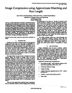
V. JPEG BASELINE CODING VERSUS TCHEBICHEF TRANSFORM COMPRESSION JPEG is an international compression standard which is designed to support a wide variety of applications for continuous-tone images. JPEG baseline which is based on DCT is a lossy technique commonly used today and is sufficient for a large number of applications [1]. Using the JPEG Compression platform, 8×8 forward DTT has been used inplace of DCT. Fig. 2 shows how the FDTT is performed on the 8×8 blocks of image data in order to achieve good compression performance.
From (13) and (14) it is clear that 2-D DTT and 2-D DCT are just one dimensional DTT and DCT applied twice by successive 1-D operations, once in x-direction, and the once in y-direction. B. Even Symmetry From [4], it can be shown that Tchebichef polynomials satisfy the property t p ( N − 1 − x) = (−1) p t p ( x),
p = 0,1,....N − 1.
(15)
For DCT:
Forward DTT
Quantization Process
Entropy Encoding
Zig zag Ordering
Input 8×8 image blocks m
C m (n) = (−1) C m ( N − n − 1), m = 0,1,....N − 1.
(16) Compressed output data
The above two properties are commonly used in transform coding methods to get substantial reduction in the number of arithmetic operations.
Fig. 2. Implementation of FDTT on the 8×8 blocks of image data.
C. Orthogonality DTT and DCT basis functions are orthogonal. Therefore, this property renders some reduction in the pre-computation complexity. Fig. 1 (a) and (b) shows the 2-D basis images for the DTT and DCT. In the basis images, it has been observed that the low frequencies reside in the upper left corner of the spectrum, while the high frequencies are in the lower right. The basis functions for rows are increasing frequencies in horizontal directions while the basis functions for columns are increasing frequencies in vertical directions.
(a)
To apply FDTT, the image is divided into 8×8 blocks of pixels. The 8×8 blocks are processed from left-to-right and from top-to-bottom. After transformation, two issues namely; quantization process and entropy coding are discussed below. A. Quantization Quantization is a process which removes the high frequencies present in the original image. This is due to the fact that the eye is much more sensitivity to lower frequencies than to higher frequencies. This is done by dividing values of high indexes in the vector (the amplitude of higher frequencies) with larger values. Values of low indexes are divided with amplitudes of lower frequencies. We have used the standard JPEG luminance quantization table in [1]. B. Entropy Huffman Coding After the transformation and quantization over an 8×8 image sub-blocks, the new 8×8 sub-block shall be reordered in zigzag scan into a linear array. The first coefficient is the DC coefficient and the other 63 coefficients are AC coefficients. Because the DC coefficient contains a lot of energy, it has usually much larger value than AC coefficients. Since there is a
(b)
Fig. 1. Two dimensional Basis Image for (a) DTT, (b) DCT .
106
very close relation between the DC coefficients of adjacent blocks, the DC coefficients are differentially encoded. This process further reduces entropy. In our experiment we use basic entropy coding process. The entropy coding process consists of Huffman coding tables as recommended in JPEG standard [1]. These tables are stored as header information during the compression process so that, it is possible to uniquely decode the coefficients during decompression process.
In order to evaluate the compression performance between DTT and DCT, around 20 various kinds of images have been tested. We have observed that, for images having high intensity variations, DTT always performs better than DCT in terms of PSNR, MSE and number of AC and DC coefficients.
VI. SIMULATION RESULTS AND ANALYSIS The superiority of the proposed technique is demonstrated through computer simulation running on Microsoft Window XP, Intel Core2 Duo CPU, 3 GHz Platform. The PSNR is a metric used for comparison. PSNR is expresses as: ⎛ 255 2 ⎞ ⎟, PSNR = 10 log10 ⎜ ⎜ MSE ⎟ ⎝ ⎠
(a)
(b)
Fig. 3. Test images use for Experiment (a) Lena, (b) Slope.
(17)
33
where
dtt dct
32
1 M ×N
M −1N −1
∑∑ ( X ij − X 'ij ) 2 .
31
(18)
30
i =0 j = 0
PSNR(dB)
MSE =
'
Symbols X ij and X ij are original and reconstructed pixel values at the location ( i , j ) respectively. M × N is the size of the image. The experimental inputs for the proposed method are Lena and Slope images as shown in Fig. 3 (a) and (b) respectively. All the image dimensions are of 256×256. Fig. 4(a) and (b) shows the comparison plot (PSNR Vs Compression Ratios) of Lena and Slope images respectively. Comparison is made between proposed 8×8 DTT algorithm and JPEG, which uses 8×8 DCT algorithm. From Fig. 4(a), it is clear that the PSNR of DTT and DCT differ by almost less than 0.2 dB, for any compression ratio. Fig. 4(b) shows that the PSNR of DTT reconstructed Slope image is better that DCT at any compression ratio. In Table 1(a) and (b), a quantitative comparison is made between compression ratios (CR), Number of AC plus DC coefficients, PSNR and MSE between DTT and DCT reconstructed Lena and Slope images respectively. The ‘Scaling factor’ values indicated in the first column of Table 1, is the multiplication factor to scale the quantization matrix as described by [1]. For Lena image, it can be seen from Table 1 that, at a CR of 9.0 DCT needs around 300 less coefficients than DTT. But for higher CR DTT always needs lesser number coefficients than DCT. It can be also note that, from Table 1, DTT shows higher compression performance than DCT in most of the cases for Lena image. Furthermore, in case of Slope image, DTT shows always better compression performance than DCT, except at a CR of 35 to 37 as shown in Fig 4(b). This fact is also clearly evident form the second line of Table 1 in case of Slope image. For the same image case, the AC plus DC coefficients at a CR of 35 to 37, are around 200 bits more in DTT than DCT. But other CR DTT needs fewer coefficients than DCT.
29 28 27 26 25 24 23
5
10
15
20
25 30 Compression Ratio
35
40
45
50
(a) 40 dtt dct
PSNR(dB)
35
30
25 15
20
25
30
35 40 45 Compression Ratio
50
55
60
(b) Fig. 4. PSNR-Compression Ratios curve between DTT and DCT of (a)Lena, (b) Slope image.
107
TABLE I COMPARISON OF COMPRESSON RATIO (CR), NUMBER OF DC AND AC COEFFICIENTS, PSNR (dB) AND MSE BETWEEN DTT AND DCT 1. Lena Image: Scaling factor
DTT(Proposed) CR
1 5 10 15
9.0 24.63 37.72 46.92
No. of bits to encode DC coefficients
No. of bits to encode AC coefficients
5790 4087 3704 3538
51854 17196 10194 7635
Total DC & AC Coefficients (in bits) 57944 21283 13898 11173
DCT(Used in JPEG) PSNR
32 27 25 23
MSE
CR
37 119 209 306
9.0 24.49 37.57 46.89
No. of bits to encode DC coefficients
No. of bits to encode AC coefficients
5789 4088 3705 3540
51854 17318 10252 7640
Total DC & AC Coefficients (in bits) 57643 21406 13957 11180
PSNR
33 28 25 23
MSE
34 112 203 300
2. Slope Image: Scaling factor
DTT(Proposed) CR
1 5 10 15
19.52 36.28 50.06 54.86
No. of bits to encode DC coefficients 5568 4342 3754 3550
VII.
No. of bits to encode AC coefficients 21286 10110 6721 6006
DCT(Used in JPEG)
Total DC & AC Coefficients (in bits)
PSNR
MSE
CR
26854 14452 10475 9556
39.2 31.36 27.64 25.69
7.83 47.60 112.1 175.7
19.32 36.86 49.82 55.04
CONCLUSIONS
[7]
REFERENCES [2] [3] [4] [5] [6]
5567 4342 3754 3550
No. of bits to encode AC coefficients 21571 9879 6771 5976
Total DC & AC Coefficients (in bits)
PSNR
MSE
27138 14221 10525 9526
38.9 31 27.3 25.67
8.36 51.3 122 176
R.Mukundan and O.Hunt, “ A comparison of discrete orthogonal basis functions for image compression”, Proceedings Conference on Image and Vision Computing New Zealand IVCNZ 2004, pp. 53-58. [8] Wong Siaw Lang, Nur Azman Abu and Hidayah Rahmalan, “Fast 4x4 Tchebichef Moment Image Compression”, socpar, pp. 295-300, 2009 International Conference of Soft Computing and Pattren Recognition, 2009. [9] S.Ishwar, P.K.Meher and M.N.S.Swamy, Discrete Tchebichef Transform- A Fast 4×4 algorithm and its application in Image/Video Compression”, ISCAS 2008, May 18-21, pp.260-263, USA 2008. [10] S.A.Abdelwahab, “Image Compression using Fast and Efficient DiscreteTchebichef Algorithm”, In Proc of INFOS 2008, The 6th International Conference on Informatics and Systems, Cairo, Egypt, March 27-29, 2008, pp. 49-55. [11] I.E.Richardson, H.264 and MPEG-4 Video Compression. John Wiley and Sons, 2003.
In this paper, an 8×8 DTT algorithm is implemented in the JPEG in place of 8×8 DCT algorithm. By using various test images, it has been observed that DTT has energy compaction property competitive with that of DCT and thereby provides compression performance relatively close with DCT. Therefore, it can be a suitable candidate for applications such as PDAs, mobile phones and digital cameras where efficient image compression techniques are required. The proposed work is implementation of 8×8 DTT algorithm using Matlab. Future research work in this field is to develop a DTT fast algorithm for input block of size 8×8. [1]
No. of bits to encode DC coefficients
W.B.Pennebaker and J.L.Mitchell, “JPEG Still Image Compression Standard”, Chapman & Hall, New York,1993. R.Mukundan “Radial Tchebichef Invariants for Pattern Recognition”, In Proc of IEEE TENCON’05 Conference, Melboroune, 21-24 Nov. 2005, pp. 2098-2103(1-6). K.Nakagaki and R.Mukundan, “A Fast 4x4 Forward Discrete Tchebichef Transform Algorithm,” IEEE Signal Processing Letters, vol.14, no.10, October 2007. R.Mukundan, “Some Computational aspects of Discrete Orthonormal Moments”, IEEE Transaction on Image Processing, vol. 13, no.8, pp. 1055-1059, Aug 2004. R.Mukundan, “Image Analysis by Tchebichef Moments”, IEEE Trans. on Image Proc., vol.10, no.9, pp.1357-1364, 2001. Nur Azman Abu, Nanna Suryana and R.Mukundan, “ Perfect Image Reconstruction using Discrete Orthogonal Moments”, Proceedings of the 4th IASTED International Conference on Visualization, Imaging and Image Processing VIIP 2004, pp.903-907, 6-8 Sep 2004, Marbela, SPAIN.
108