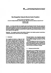
TRANSFORM CODING USING DISCRETE TCHEBICHEF POLYNOMIALS R. Mukundan Department of Computer Science and Software Engineering University of Canterbury Christchurch New Zealand.
[email protected] ABSTRACT Moment functions based on Tchebichef polynomials have been used recently in pattern recognition applications. Such functions have robust feature representation capabilities needed for a recognition task. This paper explores the possibility of using orthonormal versions of Tchebichef polynomials for image compression. The mathematical framework for the definition of Tchebichef transforms is given, along with the various analytical properties, recurrence relations and transform equations. Initial experiments with gray level images have yielded promising results, with the Tchebichef transform giving a higher PSNR value compared to the cosine transform for certain image reconstructions. KEY WORDS Discrete Orthogonal Polynomials, Tchebichef Polynomials, Image Reconstruction, Image Compression, Discrete Cosine Transform.
1. Introduction Moment functions based on discrete orthogonal polynomials have been recently used as shape descriptors in computer vision applications [1,2]. Orthogonal moments provide better feature representation capability and improved robustness with respect to image noise, over other types of moments [3-5]. Commonly used basis functions for these applications are the discrete Tchebichef (Chebyshev), Hahn, and Krawtchouk polynomials. The Tchebichef polynomials have unit weight and algebraic recurrence relations involving real coefficients, which make them suitable for defining image transforms for compression and reconstruction. Discrete Cosine Transforms (DCT) are widely used in the area of signal processing, particularly for transform coding of image data. The 8-point DCT is the basis of the JPEG standard, as well as several other standards such as MPEG-1 and MPEG-2. The basis vectors of the DCT are derived from the class of discrete Chebyshev polynomials [6], which are defined as follows.
1
T0 (i ) =
N
,
i = 0,1,…, N−1.
2 cos( p cos −1 ξ i ) , N p = 1,2,…, N−1, i = 0,1,…, N−1.
T p (ξ i ) =
where
(1)
Tk (ξ i ) is the kth Chebychev polynomial.
Substituting
ξ i = cos
(2i + 1)π , 2N
i=0,1,2,…, N−1,
(2)
in (1), the basis functions for the DCT are obtained as follows [6,7]:
τ 0 (i ) = τ p (i ) =
1 N
,
i = 0,1,2,…, N−1,
2 ( 2i + 1) pπ , cos N 2N p = 1,2,…, N−1, i = 0,1,2,…, N−1.
(3)
The above discussion points to a close mathematical relationship between the coefficients of a Chebyshev transform and the Discrete Cosine Transform. This motivates us to consider other types of discrete Chebyshev polynomials that are suitable for similar applications in signal and image processing. For example, the Tchebichef moments in [1] are defined based on a set of kernel functions which satisfy the following recurrence relations: T0(i) = 1 T1(i) = 2i + 1− N (p+1)Tp+1(i)−(2p+1)(2i+1−N)Tp(i)+p(N2−p2)Tp−1(i)= 0, p=1,2,…,N−1, i=0,1,…,N−1. (4) The orthonormal versions of the above set of polynomials are particularly useful for feature representation, image
reconstruction, and recognition. This paper examines the transform properties of the above class of polynomials, and shows that they can be applied in image compression algorithms. Experimental results show a close similarity between the performance of the Discrete Cosine Transform and Tchebichef transform. For certain gray level images, the Tchebichef transform provides a better reconstruction error than the DCT. The paper is organized as follows: The next section gives the mathematical framework for defining orthogonal Tchebichef transforms, and presents the corresponding basis images and transformation matrices. Section III outlines the important transform properties that are useful in a compression algorithm. Section IV presents the results of a several experiments carried out using graylevel images.
2. Orthonormal Tchebichef Polynomials The orthonormal version of the one-dimensional Tchebichef functions in (4) is given by the following recurrence relations in polynomials tp(x) of degree p defined on a discrete domain x = 0,1,… N−1: t p ( x ) = (α 1 x + α 2 ) t p −1 ( x ) + α 3 t p − 2 ( x ) , p=2,..N−1
(5)
N −1
∑ t p ( x)t q ( x) = δ ( p − q)
x =0 N −1
(8)
∑ t p ( x)t p ( y ) = δ ( x − y )
p =0
At this stage, it is worthwhile comparing the recurrence relations for Tchebichef polynomials as given in (5) with that of the Discrete Cosine Transform: (2i + 1)π τ p −1 − τ p −2 , 2N p = 3,…,N−1, x = 0,1,…,N−1.
τ p ( x) = 2 cos
(9)
where the starting values (for p=1,2) of the DCT recurrence relation are given by (3). For more details on the definition of Tchebichef polynomials, see [8,9]. Some of the computational aspects related to the evaluation of Tchebichef polynomials of large degrees are discussed in [10]. In this paper, we propose a compression algorithm similar to a 8-point DCT, based on an image transform requiring only polynomials of degree 0 through 7: 7
7
Tpq= ∑ ∑ t p ( x)t q ( y ) f i ( x, y ) , p, q, x, y=0, 1,..7. (10) x =0 y =0
where
α1 =
α2 =
The inverse transformation of Eq. (10) has the form
2 p
2
4 p −1 N 2 − p2
,
f(x, y) =
2
N −p
2
( p − 1) p
2 p +1 2p −3
N 2 − ( p − 1) 2 N 2 − p2
1 N
.
(6)
3 N ( N 2 − 1)
.
7
,
p, q = 0, 1, 2…7.
(12)
where each 8×8 matrix Bpq (called a basis image) is defined as
B pq
,
t1 ( x) = (2 x + 1 − N )
7
∑ ∑ T pq B pq (i, j )
p = 0 q =0
The starting values for the above recurrence relation can be obtained from the following equations: t 0 ( x) =
(11)
Eq.(11) can also be expressed using a series representation involving 82 matrices as follows [11]:
,
f(i, j) =
α3 =
7
p =0 q =0
4 p2 −1
(1 − N ) p
7
∑ ∑ T pq t p ( x)t q ( y )
(7)
The functions {tp(x)} satisfy the following properties of orthogonality and completeness:
t p (0)t q (0) t p (0)t q (1) L t p (0)t q (7) t (1)t (0) t (1)t (1) L t (1)t (7) p q p q p q , = L L L L t p (7)t q (7) t p (7)t q (0) t p (7)t q (1)
(13)
The complete set of 64 basis images for the discrete Tchebichef polynomials is given in Fig. 1.
β1 =
− p ( p + 1) − ( 2 x − 1)( x − N − 1) − x x( N − x)
β2 =
( x − 1)( x − N − 1) . x( N − x)
(16)
Also, t p ( 0) = −
N−p N+p
2p +1 t p −1 (0) , 2 p −1
p = 1,…N−1. (17)
The above recurrence formulae are useful especially when Tchebichef polynomials of large degree are required to be evaluated [10]. The basis set of the DCT provides a good approximation to the eigen vectors of the symmetric Toeplitz matrices defined as [6,7]:
Figure 1. 8×8 basis images of orthonormal Tchebichef polynomials For comparison, the values of DCT polynomials τp(i), and Tchebichef polynomials tp(i), for p=0,…7, i=0,…3 are given in Table 1. Discrete Cosine Transform
1 ρ ψ = ρ2 M ρ N −1
1
ρ2 ρ
ρ
1
ρ
ρ
M
N −2
ρ
M
N −3
L ρ N −1 L ρ N −2 L ρ N −3 M 1
(18)
The orthonormal Tchebicef polynomials also satisfy the above property, and the plots of the Tchebichef polynomials values (solid lines) and the eigenvectors of Ψ for N=8 and ρ=0.95 (dotted lines), are given in Fig. 2
0.35355 0.35355 0.35355 0.35355 0.49039 0.41573 0.27779 0.09755 0.46194 0.19134 -0.19134 -0.46194 0.41573 -0.09755 -0.49039 -0.27779 0.35355 -0.35355 -0.35355 0.35355 0.27779 -0.49039 0.09755 0.41573 0.19134 -0.46194 0.46194 -0.19134 0.09755 -0.27779 0.41573 -0.49039 Discrete Tchebichef Transform 0.35355 0.35355 0.35355 0.35355 -0.54006 -0.38576 -0.23146 -0.07715 0.54006 0.07715 -0.23146 -0.38576 -0.43082 0.30773 0.43082 0.18464 0.28204 -0.52378 -0.12087 0.36262 -0.14979 0.49215 -0.36377 -0.32097 0.06155 -0.30773 0.55391 -0.30773 -0.01707 0.11949 -0.35846 0.59744
Table 1. Values of DCT and Tchebichef polynomials for N =8.
3. Transform Properties The Tchebichef polynomials in (5) satisfy the symmetry property given by the equation t p ( x) = (−1) p t p ( N − 1 − x) ,
x=0,1,….N−1.
(14)
The above property is also evident from the values given in Table 1. In addition, tp(x) also satisfies a recurrence relation in the variable x:
t p ( x ) = β 1 t p ( x − 1) + β 2 t p ( x − 2) , p=1,…N−1; where
x = 2,3,… N.
(15)
Figure 2. Comparison of orthonormal Tchebichef polynomial values and the eigenvectors of the Toeplitz matrix.
4. Experimental Results This section provides a comparative analysis of the performance of the DCT and the DTT, using a set of standard gray-level images. The images are first partitioned into non-overlapping blocks of 8x8 pixels. Using the 8x8 transformation matrix ‘A’ of the polynomial values, each image block is transformed into a block of coefficients (Fig. 3). A traversal through the 64 coefficients in a zig-zag pattern (used in JPEG compression) is performed to progressively reconstruct the image from 1 to 64 coefficients.
Figure 3. 8x8 block of coefficients with the zig-zag pattern. We use the peak signal-to-noise ratio (PSNR) as the normalized error measure to define the quality of the reconstructed image. The PSNR value is given by PSNR = 10 log10
255 2 , MSE
(19)
where MSE denotes the mean square error of the reconstructed image with respect to the original image. Fig. 4 shows a set of images used in our study. The polynomial values are computed using the recurrence relations given in equations (15)-(17). The images are selected in such a way that they have significantly different values of Spatial Frequency Measures (SFM) and Spectral Activity Measure (SAM) as these are image quality measures commonly used for testing the performance of compression algorithms [12].
Figure. 4. Set of images used in the experimental evaluation of the Tchebichef transform The SFM and SAM values computed for the above set of images are given in Table 2.
Image N SFM SAM Lenna 256 20.0813 481.1971 Stripes 256 15.9978 33095.8027 Fingerprint 256 23.3546 6766.2199 Boat 512 17.8687 1131.4111 Baboon 512 36.5393 99.3261 Ruler 512 116.8405 384.6774 Table 2. SFM and SAM values of images in Fig. 4.
The PSNR values computed from the reconstructions of the above set of images for both the DCT and the DTT are plotted in Figs. 5,6.
Figure 5. Comparison of reconstruction errors for Lenna, Stripes, and Boat images.
Figure 6. Comparison of reconstruction errors for Fingerprint, Baboon, and Ruler images It is not difficult to notice that the discrete Tchebichef transform gives a better reconstruction (higher PSNR value) for images ‘Ruler’, ‘Stripes’, and ‘Fingerprint’. The ‘Stripes’ image has high predictability and large intensity gradients. Regions of large gradients are also present in the ‘Ruler’ image. The ‘Fingerprint’ image on
the other hand contains regions of high frequency. The images ‘Lenna’, ‘Boat’, and ‘Baboon’ have low predictability compared to other images. In general the discrete Tchebichef transform gives a better performance for images with sharp boundaries, and high predictability.
[7] N. Ahmed, K.R. Rao, Orthogonal transforms for digital signal processing (Springer-Verlag, 1975).
5. Conclusion
[9] Nikiforov A.V, Suslov S.K, Uvarov V.B, Classical orthogonal polynomials of a discrete variable (Springer-Verlag, 1991).
This paper has introduced the Discrete Tchebichef Transform (DTT) as a possible alternative to DCT for applications in image compression and reconstruction. The Tchebichef transform has properties that are very similar to that of the DCT. This can be clearly seen in the basis images and the transform matrices. The paper has presented the fundamental properties and the mathematical framework of the Tchebichef transform. The Tchebichef transform involves only algebraic expressions and can be computed easily using a set of recurrence relations. Experimental results have shown that the DTT can provided distinctively better reconstruction compared to DCT for images that have large intensity gradients, such as paintings and line drawings. DTT could also be used for compression by following the transformation process by quantization and Huffman coding. This procedure would be exactly similar to the DCT based compression and reconstruction.
References [1] R. Mukundan, S. H. Ong, P. A. Lee, Image analysis by Tchebichef moments, IEEE Trans. Image Processing, 10(9), 2001, 1367-1377. [2] P.T. Yap, R. Paramesran, S.H. Ong, Image analysis by Krawtchouk moments, IEEE Trans. Image Processing, 12(11), 2003, 1357-1364. [3] M. R Teague, Image analysis via the general theory of moments, J. Optical Soc. Of America, 70, 1980, 920-930. [4] R. Mukundan, Discrete Orthognal Moment Features Using Chebyshev Polynomials, Proc. Intnl. Conf. on Image and Vision Computing - IVCNZ’00, New Zealand, 2000, 20-25. [5] R. Mukundan, S.H.Ong, P.A.Lee, Discrete vs. Continuous Orthogonal Moments in Image Analysis, Proc. Intnl. Conf. On Imaging Systems, Science and Technology CISST’2001, Las Vegas, 2001, 23-29. [6] N. Ahmed, T. Natarajan, K.R. Rao, Discrete Cosine Transform, IEEE Trans. on Computers, 23, 1974, 9093.
[8] Erdelyi, A. et al , Higher transcendental functions Vol. 2 (New York: McGraw Hill, 1953).
[10] R. Mukundan, Some Computational Aspects of Discrete Orthonormal Moments, IEEE Trans. Image Processing, 13(8), 2004, 1055-1059. [11] A.K. Jain, Fundamentals of digital image processing (Prentice Hall, 1988). [12] Grgic, S., Mrak, M., Grgic, M., Comparison of JPEG Image Coders, Proc. 3rd International Symposium on Video Processing and Multimedia Communications, VIPromCom-2001, Zadar, Croatia, 2001, 79-85.