The prediction error pattern e(i,j) is therefore an m-level pattern, with few non-zero ..... munication, John Wiley & Sons, Inc., New York, 1968. 2. L. R. Bahl and H.
H. Kobayashi L. R. Bahl
Image Data Compression by Predictive Coding I: Prediction Algorithms Abstract: This paper deals with predictive coding techniques for efficient transmission or storage oftwo-level (black and white) digital images. Part I discusses algorithms for prediction. A predictor transforms the two-dimensional dependence in the original data into a form which can be handled by coding techniques for one-dimensional data. The implementation and performance of a fixed predictor, an adaptive predictor with finite memory, and an adaptive linear predictor are discussed. Results of experiments performed on various types of scanned images are also presented. Part I1 deals with techniques for encoding the prediction error pattern to achieve compression of data.
Introduction
164
Data sources such as facsimile transmission signals and digitized images to be stored in a computer memory contain a substantial amount of redundancy. Source coding [ I ] techniques(also called datacompactionor compression) can be used to efficiently encode the outputs of such sources. There are two obvious applications of these compression methods. The first is in communication systems. By encoding the source, we can transmit the information over acommunicationchannel in a shorter time period.Alternatively, wecould use a channel with a smallerbandwidth totransmitthecodeddata (hence the often used term “bandwidth compression”). The second application is in storage systems, which can be used more efficiently by reducing the amount of data to be stored. In this paper we discuss some theory and methods for compressingtwo-dimensional black andwhiteimage data through the use of predictive coding. Part I1 [2] describes encoding techniques designed to achieve compression.Before going intodetailed discussions on the particular approaches taken, we briefly review some of the recent progressin the general area of image compression. Techniques in the art of compressing two-dimensional image data can be classified into two categories: 1) time-domain (orspace-domain) encoding and2) transform-domain encoding. The time domain techniques that appear practical are mostly of the prediction-comparison type. Thisincludes schemes like delta modulation and differential pulse code modulation [3]. Most studies of such systems arebased on theclassical communication theory approach. The first information theoretic treat-
H. KOBAYASHI AND L. R. BAHL
ment of this subject was done by Elias [4], who called the technique “predictive coding.” In predictive coding the dependence inherentin the data canbe removed by a good predictor that transforms the original data into a form such that successive data symbols are nearly independent of each other. The transformed data can then be encoded by techniques applicable to independent sources. Application of predictive coding to compression of pictorial data hasbeen reRorted by Wholey [ 51 and by Arps [ 61. Recent results in the theory of data compression systems that use prediction and interpolation have been discussed by Balakrishnan [7] and by Davisson [8]. Applications of theirstudies to weather satellite pictures are reported by Kutz and Sciulli [9]. The transform-domain methods [ 10- 121 include the application of Fourier,Hadamard-Walsh, KarhunenLoeve,andother transforms. In all thesemethods a block of data samples is decomposed into a set of coefficients of orthogonal functions, and the coefficients are transmitted. Compression of’data is obtained by eliminating insignificant coefficients or by reducing the number of levels of quantization i n the transform domain. There is, of course,some degradation in thereconstructed image. With the advent of fast transform’ methods 13 151 thatare particularlysuited for high-speed digital computers, the transform techniques have recentlyreceived considerable attention. Forcomprehensivetreatments of thesubject,the reader is referred totherecently published books by Huang and Tretiak [ 161, Andres [ 171, and Rosenfeld [ 181, and to a specialissue of journal papers[ 191.
IBM I. RES. DEVELOP.
. .
Image-data compression systems with predictive coding
In the present work our main interest lies in efficient source coding of two-dimensional digital image data, i.e., data from sources that are discrete both in space and in amplitude [20]. Typical examples arethe quantized values of facsimile scanner output and graphic display data of computer systems. We limit ourselves to those cases where the amplitude is quantized to just two levels. Figure 1 illustrates a communication system that uses predictjve'coding. Assume a two-dimensionaldata source s(i, j ) , 1 5 i 5 i, 1 5 j 5 J , in which the value of each pictureelement (pel) s can be either 0 (white) or 1 (blackj. We can expect value the of pel s (i, j ) to beclosely related to the values of its neighboring pels, s ( i - 1, . j - l ) , s ( i - l , j ) , s ( i - l , j + I), s ( i , j ~1);etc. (Fig. 2 ) . It is therefore possible to predict s (i, j ) with a high probability of success from the values of neighboring pels. This is the function of the predictor in Fig. 1: The set of point; on which the predictor bases its prediction of the generic pel ( i , j ) is called the memory set M of the predictor. For example, in the caseof tbe +pel predictor of f . Fig. 2 , the memory set is
1 Figure 1 An image datacompressionsystem coding and decoding.
s( i-1,j-I)
s(i-l,j)
with predictive
s(i-l,j+l)
M = {s(i- i , j - l ) , s ( i - l , j ) , s ( i -I )l,, j +
s(i,j-
1)).
(1)
The output i(i, j ) of the predictor module is compared with the actual value s ( i , j ) and an error signal e ( i , j ) is derived from the operation e ( i , j ) = s ( i , j ) @ t(i,j),
Figure 2 Two-dimensional data and their prediction based on the neighbors.
(2)
to thoseof the predictor at the transmitter side. The s (i, j ) where @ means modulo 2 addition, an operation thatcan are reconstructedaccording to the inverse rule of ( 2 ): be realized by an EXCLUSIVE OR circuit. s(i,j)= e(i,j) @t(i,j). (3 1 If the 'tyo-dimensional data s (i, j ) . are read by raster scanning,they are transformed into aone-dimensional The system represented by Fig. 1 can be extended to time series denoted by s (n),'where n = ( i - 1 )J + j and multilevel (grey level) signals, e.g., the case in which the 1 f n 5 ZJ. The sequence s ( ~ is ) first read into a buffer s ( i ,j ) take on m different levels, 0, I , . . ., m - I . The mod 2 additions in ( 2 ) and (3 ) should then be replaced memory. The 4-pel predictor of Fig. 2 is given at time by mod rn subtraction and mod m addition, respectively. n thevalues s(n- 1); s ( q - J l ) , s(n - J ) , and The prediction error pattern e ( i , j ) is therefore anm-level s ( n - J - 1 ) from the memory and it generates s*(n),a predicted value of s (n). The original data s (i, j ) tend to pattern, with few non-zero values, since most predictions be higlily redundant so most predictions are found'to be will be correct. correct. This results in an error pattem e ( n ) [or equivaThe information in the error signal e ( i , j ) is precisely lently e ( i ,j ) 3 which is very sparsein binary 1's. the information in the original image s ( i , j ) because either The errorsignal is encoded by some'efficient data comcan be obtained uniquely from the other. Note that prepression scheme andis then transmitted or put into a data dictionby itself does not achieveany compression. However, a substantial difference in the efficiency of storage system. At thereceiving end, or in retrieving the data froma storage system, the decoder recovers the errorcoding may occur depending on whether one encodes s ( i ,j ) or e ( i ,j ) . An efficient code for s ( i ,j ) would resignal from its encoded form and the original data are require that a large number N of pels be encoded simulconstructed by passing e ( i , j ) into a circuit that cmtainsa taneously. This imposes tworequirementsonthe enpredictor in its feedback loop (Fig. 1). The structure of coding: this predictor and its prediction ?le should be identical
+
MARCH
1974
165
IMAGEDATACOMPRESSION
i'L'#'l'l'l' s(n-1)
Updating of predictionrule
s(n"l+l)
s(n-J)
s(n-J-I)
s(i,i)
Figure 3 An image datacompressionsystemwithadaptive
Figure 4 Adaptive linear threshold logic predictor with N = 4.
predictor.
1. There must be an active memory that stores the past N or more terms of s ( i ,j ) . 2. There must be a codebook memory that lists the codewords for all possible patterns of N terms. The number of entries in the codebook is 2N. Furthermore, if each block is encoded independently, the inherent dependence between adjacent blocks is not exploited. In predictive coding, on the other hand, the error sequence e ( i , j ) is, in most cases, approximated by the output of a memoryless (zero-memory) source because the serial (or spatial) redundancy is removed by the predictor. As discussed in Part 11, this latter result allows convenient encoding of data without resorting to a large codebook. Prediction algorithms
166
H.
Predictors and criterion for optimality One problem in the design of a predictor is the choice of the memory set. Clearly, points adjacent to the point to be predicted are the most useful and should be contained in the memory set. We also restrict the memory set to contain points that have been scanned prior to the pointcurrently being predicted. (It is possible to construct look-ahead predictors which violate theabove constraint, but the advantages,if any, of such predictors have not been investigated.) It is advantageous to have as large a memory set as possible, but since the complexity of the predictor grows with the size of the memory set, practical considerations generally limit the memory set to contain only a few points, generally less than10. For a given memory set, the"best predictor" is defined as one that requires theminimum number of bits for the a transmission of its error pattern. However, we need more specific definition to get meaningful results. The
KOBAYASHI AND L. R. BAHL
purpose of predictive coding is to remove the redundancy from the image pattern. If the predictor does a good job of redundancy removal the error pattern can be considered to be a completely random pattern. If we make the assumption that the error pattern is truly random, the compression obtained by encoding the error pattern is determined onlyby the prediction error probability. Therefore we choose the minimization of prediction error probability as our criterion of optimality. In practice, a predictor does not remove all of the redundancy in the image, only a substantial portion of it. Consequently the error pattern is not completely random. However, to be random isthe most assuming theerrorpattern pessimistic assumption and it gives us a lower bound on the performance of the compression system. Another justification for choosing the minimization of prediction error probability as the optimality criterion is its practicality in analysis and implementation. Dejnition A predictor is called optimum if the prediction error terms e ( i, j ) [or e( n ) ] contain, on the average, the least numberof l's, which identify prediction errors.
If the size of the memory set is N (i.e., an N-pel predictor), the set can take on 2N different states (or values) which we denote by M,, k = 1, 2; ' ., 2N. Fixed predictors Assume that the data sequence is stationary and we are given the conditional probability q( 1/ M , ) = Pr{s = 1 /memoryset = M , } ,
(4)
for all k = 1, 2; . ., 2". We further assume thatprediction is performed pel-by-pel according to a fixed prediction rule. Then we obtain the following theorem for anoptimal fixed prediction rule.
IBM J . RES.
DEVELOP.
Theorem I If the memory set takes on state M k , then
0 if q( 1IM,) < 0.5; 1 if q( 1 IM,) 1:0.5. The minimized probability of prediction error is given by
fl
P,=
I:r ( M , ) min {q(1lhfk),
1 - q(llMk)},
(6)
Figure 5 Typical behavior of C,.
k=l
where r(M,) = Pr {memory set = M,}.
(7)
The proof of the above theorem is given by a straightforward application of the well-knownBayes'decision rule[20].Inactual applications q( 1 I M,) should be obtained empirically. The appropriate choice of a memory set must be left to the designer's judgment since there seems to be no general way of defining an optimal memory set. However, one can see intuitively that performance would be improved by expanding any given memory set. This, in fact, can be proven under the same assumption made in the theorem. We state this fact as a separate theorem. Theorem 2 The probability of prediction error of an optimal fixed. predictor is not increased by expanding the memory set.
The formal proof is given in [20] and is lengthy; it is based on the concave property of the function f (x) = min (x,1 - x). One of the disadvantages of a fixed predictor is that the size of the decision table grows exponentially with N , and hence its dimension becomes huge when N gets large. It is possible to reduce the predictor complexity to some extent byapplying techniques from switching theory,suchas Karnaughmaps [21 I orthe QuineMcClusky reduction method [221. Adaptive predictors A fixed predictor of the type discussed aboveis justified if the statistics of the data [i.e., q( 1 IM,)] are known or available in advance (e.g., by prescanning)and if the data from the source are stationary. The adaptive predictors providesolutions thatare practicalwhen data or nonstationary.Theuse of statisticsareunknown theseadaptivepredictorsrequiresnoextra channel space: The predictor at the receiver operatesin exactly the same manner as the one at the transmitter side, and updating of its prediction rule can be done synchronously with that of thetransmitterbecausetheadaptation is controlled by the signal s( i, j ), which is available at both ends of the system (Fig. 3). Adaptive threshold-logic predictor The predictor outputs^ forms a finite set of discrete levels
MARCH
1974
(0 and 1 in our case), so any of the pattern classifier or discriminant functions can be used as a predictor [23 1. The simplest type of adaptive classifier is a linear learning machine or adaptive threshold logic unit (TLU). Let {x1, x2,. . ., x,} be values of data in the memory set of dimension N . For example, in the caseof the 4-pel predictor of Fig. 4. these x's at time n are
x,= s ( n - l ) , x, Define an ( N
= s(n - J
+ l ) , x3 = s ( n - J ) , and x4 = s ( n "J + 1).
(8)
+ 1)-dimensional vector x by
x = (1, XI, xz;. .>x*,),
(91
and consider the following linear function of the vector: N
+ wo = (w, x), where w is an ( N + 1)-dimensional vector, F (x) = i=1 wixi
w = (wo, W1'
wz3.
. .>WN),
(11)
and the wi'sare real numbers. For practical purposes the wi's can be integers. This condition is met automatically if the initial values of w and a of ( 13) are integers. Then the prediction is done according to the following simple rule:
This linear predictor can be made adaptive by the following rule: The initial choice of the weight vector w may have any value. The w is modified only when the prediction fails. That is, let the new weight vector w' be w'=(
w + a x i f s = 1 andi=O; w-axifs=Oandi=l.
(13)
The choice a 1 0 for the coefficients determines the stability and convergence speed of the predictor. Several rules for choosing a are known [24, 251. The simplest types are a ) fixed increment rule, where (Y is any fixed positive number, and b) absolute correction rule, where a is the smallest integergreater than I (w, w) 1 / 1x1'. In itsusualapplications topattern recognition, the adaptation of this discriminant function is donein a training period that precedes the test period. Although this operational mode is also applicable to the problem at hand, we can provide a more attractive mode in our 'ap-
1617
IMAGEDATACOMPRESSION
the small computers need to be backed up, they can have a link to the large central computers. Since in many experiments the raw events can be converted easily into a more economical format, or frequently even rejected as useless afterthe simplest geometrical checks, another wayof "stretching" the capacity of the on-line computers is to perform a maximum of simple logical operations on thedata before they enter the computer. This reduces the amount of valuable memory taken up by buffers for useless information and leaves much more memory (and also time) for programs treating the useful data. The system designed for the experiment on line to the 360/44 is anattempt in this direction. Defining the center of a cluster of triggered wires in a wire spark chamber by special hardware is another.
ist, for although a huge effort went into each program, the result was usually a program extremely efficient in execution time and space usage. With the arrival of newer computers, with support of on-line applications even extending as far as time-sharing systems, the tendency has been to program in machine language only those operations which would be extremely ineficient in a higher level language, for example handling theinput/output and buffering, and to make use of the flexibility of the system and the high levellanguages for most other tasks. However, in some applications it has been found that the high overheads imposed by these systems, often written for process control applications, have put such restriction on the datataking capacity as to outweigh the advantages givenby the flexibility.
IBM J. RES. DEVELOP.
plication. That is, there is no need to set up a training period separate from the test period. We can operate this learning machine in an adaptive modeall the time without any interception or prescanning. So far we have discussed only the linear learning machine because of its simplicity. However, essentially all types of learning machines and discriminantfunctions can be used as adaptive predictors. A @ function [24] is defined by
+ w,f,(x) +...+ w,f,(x),
@(x) = w,+ w , f , ( x )
4-pel predictor
7-pel predictor
(14)
where &(x), i = 1, 2, * . ., M , are any real functions of x. For example, they can be chosen to extract important features of patterns. Another classof pattern classifiers is “layered machines” [24,25]. A layered machineis a network of TLUs, organized in layers. This class includes the piecewise-linear discriminant function machines and the “a-perceptron.” 12-pel predictor
Adaptive predictor with jinite memory In the fixed predictor discussed previously, an optimal prediction table must contain one bit of information for each stateM , of the memory set, k = 1, 2; . ., 2N.The bit indicates whether the conditional probability q ( 1/ M , ) is greater than 0.5. But prior to setting up the decision table, one needs toestimate q ( 1 / M , ) by prescanning or some other means. Now, by assigning a few extra bits to each entry of this decision table, we can develop a practical scheme that does notneed prior knowledge of data statistics. We associate with each state M , a counter C,. Let each counter haveL bits ( L 2 1) ; therefore C , can count from o to zL- 1. The predictionand adjusting algorithmsproceed as follows. For a given memory set M,, predict according to
Figure 7
Predictorsused inthe experiments.
(16)
The appropriatechoice of bit-size L for the counterC, should be a compromise between two conflicting factors: If L is small, the value of C, is susceptible to irregular or noisy data; on the other hand, if L is large, ittakes a large number of data points to reach convergence and also to accomplish a transition from oneregion to another. Manyinterestingvariations of the update algorithm (16) are possible. For example, we could make the contents of all counters decaywith time to themedian value. Or, if the behavior of certain states is correlated, we could update more than one state each time, and so on. However, we have found through experiments that the value of reducing the prediction error rate by adopting such variations is negligible in comparison with the increased complexity of the algorithms.
Typical behavior of C, is illustrated in Fig. 5 in which a two-bit counter ( L = 2) is chosen. The memory set takes a state M , at times n , , n,, n3, ’ . during which C , moves either up or down according to the rule (16). In this illustrative example a transition takes place from one region to anotherin which statistical properties of the image patterns are different: In region A q( 1/ M , ) appears to be larger than 0.5 and in region B, less than 0.5. Prediction errors occur attimes nl,3,ns, and n9. The behavior of C, can be treated as a one-dimensional random walk with reflecting barriers at C, = 0 and C, = 2L- 1 [26].
The techniques of prediction discussed in the previous section have been applied to data from three different sources: a page from the IBM Journal of Research and Development [Fig. 6(a)] and two line-drawings from a machine jobshop [Figs. 6(b) and 6(c)]. The size of the documents from which the data were obtained is 83 in. X 1 1 in. and the scanning resolution is 125 pels per inch, i.e., each pel is 8 mils (0.2 mm) square. Figure 7 lists the memory sets of the predictors used in this experimental study. When fixed predictors are used,
After the value of a pel is predicted, the actual value at that pel is used to update theup-down counter C, as follows: Its new value is min {c,+ 1, 2L- 11 [max {C,- 1,0} if
if
s = 1, s=O.
e,
MARCH
1914
Experimental results and conclusions
Type of predictor
Prediction error (percent)
7-pel finite memory adaptive ( L = 3) 7-pel fixed (prescanning) 4-pel finitememory adaptive ( L = 3 ) 4-pel fixed 12-pel adaptive linear (a= 1 ) 4-pel adaptive linear (a= 1 )
4.79 5.14 5.16 5.85 6.14 7.22
Table 2 Experimental results on machine jobshop charts (125 pels per inch).
Prediction error (percent) Type of predictor
7-pel fixed 4-pel finite-memory adaptive 4-pel fixed 12-pel adaptive linear(a= 1 ) 4-pel adaptive linear(a= 1 )
20% or more of the entire page isprescanned to derive an optimal predictor rule. Adaptive linear predictors are applied withthe initial setting w i= 0 for i= 0 , 1; . ., N and no prescanning. Finite-memory adaptive predictors start with every counter set to half its capacity, i.e., C, = 2L", k = 1, 2;*., 2N. Figure 8 shows a portion of a scanned image s (i,j ) and the corresponding prediction error pattern e ( i , j ) when a 4-pel adaptive linear predictor is used. The prediction error patterns obtained for the other types of predictors look quite similar to this example. Table 1 Summarizes the performance of the three predictors applied to the journal page image aild it clearly shows that the finitememory adaptive predictors excel for this type of image data. Figure 9 shows plots of the prediction error rate of 4and 7-pel adaptive predictors with finite memory as the counter size L is changed. The 7-pel adaptive predictor with L = 3 yields the lowest prediction rate, 4.79 percent. An adaptive linear predictor, on the other hand, does not yield high performance. This seems to indicate that the linear constraint on a predictor is too restrictive. A substantial performance improvement is achieved by enlarging the memory set from N = 4 to N = 12, but the performance is still not as good as that of the other types of predictors. Therefore, if one wants to build a learningmachine type of predictor, he should probably use piecewise-linear or polynomial predictors.
1.20
ChartA
Chart B
2.24 2.30 2.37 2.50 2.79
1.25 1.35 1.52 1.67
Table 2 summarizes the results obtained on the machine jobshop charts A and B. We observe again the superiority of the fifiite-memod adaptive predictor over the other types. The results from chart B show that the 4-pel finite memoryadaptive predictor surpasses even the 7-pel fixed predictor.
Acknowledgments
We express our thanks to L. S. Loh for his programming assistance and to D. J . Min, E. V. Eisein, K. Myer and F. Wood for providing us with the scanned data used in our simulation study. Some of the work reported in this paper was done in collaboration with our colleagues, D. I . Barnea and D. D. Grossman. We are also indebted to R. B. Arps for many stimulating discussions on the subject. Finally we express our appreciation to P. E. Green, J. Raviv and M. G. Smith for the encouragement they gave us during the course of the work.
References 1 . R. G. Gallager, InformationTheoryandReliable Communication, John Wiley& Sons, Inc., New York, 1968. 2. L. R. Bahl and H. Kobayashi, "Image.DataCompressionby Predictive Coding 11: Encoding Algorithms," ZBM J . Res. Develop., 18,172 (1974),following paper. 3. H. R. Schindler, "Delta Modulation," IEEE Spectrum 7, 69 (October 1970).
IBM J. RES. DEVELOP.
h/
4-pel finite-memory adaptive 4-pel fixed
0.05
7-pel finitememory adaptive
1 O’OI
4“
1
IL
I
I
I
I
I
2
3
4
5
6
I
-
Figure 9 Prediction error rate p e vs counter size L : experimental results from the journal page data.
4. P. Elias, “Predictive Coding, Parts I and11,” IRE Trans. Informatioh Theory IT-1,16 (March 1955). 5. J. S. Wholey, “The Coding of Pictorial Data,” IRE Trans. Information Theory IT-7,99 ( 196 1 ) . 6. R. B. Arps, “Entropy of Printed Matter at the Threshold of Legibility for Efficient Coding inDigital Image Processing,” Report No. 3 1, Stanford Electronics Laboratory, California, 1969. 7. A. V. Balakrishnan, “An Adaptive Non-linear Data Predictor,” Proc. Nut. Telemetry Conf., Washington, D.C., May 23-25, 1962, Paper No. 6-5. 8. L. D. Davisson, “The Theoretical Analysis of Data Compression Systems,” Proc. IEEE 56,176 (1968). 9. R. L. Kutz and J. A. Sciulli, “The Performance of an Adaptive Image Data Compression System in the Presence of Noise,” IEEE Trans. Information Theory IT-14, 273 (1968). 10. W. K. Pratt, J. Kane and H. C. Andrews, “Hadamard Transform Image Coding,” Proc. IEEE 57,58 (1969). 1 1 . H. C. Andrews and W. K. Pratt, “Transform Image Coding,” in Proceedings of the Symposium on Computer Processing in Communications, Polytechnic Press of the Polytechnic Institute of Brooklyn, New York, 1970, pp. 63-84.
12. H. C. Andrews and K. L. Caspari, “A Generalized Technique for Spectral Analysis,” IEEE Trans.Computers C-19,16 (1970). 13. I. J. Good, “The Interaction Algorithm and Practical Fourier Analysis,”J. Roy. Stat. Soc., Series B, 20, 361 (1958). 14. J. W. Cooley and J. W. Tukey, “An Algorithm for the Machine Calculation of Complex Fourier Series,” Math. Computation 19,297 (1965). 15. J. E. Whetchel and D. F. Guinn, “The Fast Fourier-Hadamard Transform and Its Use in Signal Representation and Classification,” EASCON Record, 1968, pp. 561-573. 16. T. S. Huang and 0. J. Tretiak (eds.), Picture Bandwidth Compression, Gordon and Breach Science Publishers, Inc., New York, 1972. 17. H. C. Andrews, Computer Techniques in Image Processing, Academic Press, Inc., New York, 1970. 18. A. Rosenfeld, Picture Processing by Computer, Academic Press, Inc., New York, 1967. 19. Special issue on “Signal Processing for Digital CommunicaCOM-19, No. 6, tions,” IEEE Trans.Communications 1971. 20. H. Kobayashi and L. R. Bahl, “Image Compaction by Predictive Coding: Fundamentals,” Research Report RC 3249, IBM Thomas J. Watson Research Center, Yorktown Heights, New York 10598, February 1971. 21. M. Karnaugh, “The Map Method for Synthesis of Combinatorial Logic Circuits,” Trans.AIEE 72, Part I, 593 (1953). 22. E. J. McCluskey, Introduction to the Theory of Switching Circuits, McGraw-Hill Book Co., Inc., New York, 1965. 23. H. Kobayashi, “Adaptive Data Compression System,” IBM Tech. DisclosureBull. 14, 1305 (197 1 ). 24. N. J. Nilsson, LearningMachines, McGraw-Hill Book Co., Inc., New York, 1965. 25. K. S. Fu, “Learning Control Systems-Review and Outlook,” IEEE Trans. Automatic ControlAC-15,210 (1970). 26. W. Feller, An Introduction to Probability Theory and Its Applications, Vol. I, 3rd ed., John Wiley & Sons, Inc., New York, 1968.
Received April 25, 1973; revisedJuly 30, 1973.
The authors are located at the IBM Thomas J . Watson Research Center, Yorktown Heights, New York 10598.
171
MARCH
1974
IMAGE DATA COMPRESSION