paper we develop a translation-invariant (TI) scheme of a general ... stage is a Laplacian pyramid (LP) that decomposes an image into a number of radial ...
IMAGE DENOISING USING TRANSLATION-INVARIANT CONTOURLET TRANSFORM Ramin Eslami and Hayder Radha ECE Department, 2120 EB, Michigan State University, East Lansing, MI 48824, USA Emails: {eslamira, radha} @ egr.msu.edu
ABSTRACT The contourlet transform, one of the recent geometrical image transforms, lacks the feature of translation invariance due to subsampling in its filter bank (FB) structure. In this paper we develop a translation-invariant (TI) scheme of a general multi-channel multidimensional FB and apply our findings to the contourlet transform to obtain a TI contourlet transform (TICT). Further, we employ the proposed TICT for image denoising, where we show that a significant improvement in the PSNR values as well as visual results is gained. Moreover, we demonstrate that this proposed denoising scheme outperforms the TI wavelet denoising approach for most experiments. We also introduce a lessredundant variety of the TICT, where we merely make the first stage of contourlets, translation invariant. We show that this transform, which we call semi-TICT (STICT), achieves a performance near that of the TICT in image denoising.
1. INTRODUCTION An important aspect of an efficient image transform is directionality. Having this feature, a transform would have the potential to handle 2-D singularities. Many directional image transforms have been introduced in recent years. Do and Vetterli introduced the contourlet transform, which is constructed using two filter bank (FB) stages [3]. The first stage is a Laplacian pyramid (LP) that decomposes an image into a number of radial subbands, and the second stage is the directional filter banks (DFB), where each LP detail subband is fed to this stage to be decomposed into a number of directional subbands. Both the LP and DFB stages involve downsampling in their analysis sections and therefore, they are shift variant. Translation invariance is a required feature in several pattern recognition applications. In addition, it is shown that using a TI version of a non-TI multiresolution framework in denoising, one can significantly improve the performance [1]. This improvement is indeed yielded from reducing Gibbs-like artifacts in the denoising results. For the wavelet transform, one can use the fast “algorithme a trous” to construct TI wavelets [6][7]. This algorithm is originally developed for a two-channel octave-band 1-D FB, which is applicable to a 1D wavelet transform. For images, this 1-D algorithm is easily extendable to 2-D wavelets using separable filters. In this work, we extend the algorithme a trous for a general case of
multi-channel multidimensional FBs to obtain TI schemes of such FBs. Then we apply the developed procedure to both stages of contourlets to realize the TICT. Since the TICT is highly redundant, we also propose the semi-TICT (STICT), where we only use a TI Laplacian pyramid (TILP) in conjunction with the (critically-sampled) DFB. We show that the STICT results in a performance for image denoising slightly lower than that of the TICT. Furthermore, we demonstrate that the TICT attains better PSNR values in most denoising experiments when compared with the TI wavelet transform (TIWT) scheme. And visually, TICT is capable of better retaining edges and textures in the denoised images.
2. DEVELOPING A TI SCHEME FOR A SUBSAMPLED FILTER BANK In this section we develop a TI variant of a general multichannel and multidimensional FB. Translation invariance is achieved through several ways. Consider a 1-D wavelet transform scheme with periodic extension, and a signal of size N. At the first level, one filters the signal using the wavelet lowpass and highpass filters, and then downsamples the resulting approximation and detail coefficients, that is, discards the odd-indexed coefficients. Now, if one cyclicshifts the signal by an even number 2k , (k ∈ Z) , the output will be the shifted version of the signal by k, that is, the single-level wavelet transform is TI for even shifts. Hence, to make this wavelet transform TI, we also need the oddindexed values of the filtered coefficients. To obtain these coefficients, one can cyclic-shift the signal by one (or an odd number) and decompose it; or, use the same signal while in downsampling shreds the even-indexed coefficients. Hence, we obtain two sets of transform coefficients for each channel (each has a size of N/2) at the first level. At the next wavelet levels, we encounter the same situation in which one shreds the odd-indexed coefficients during downsampling. Thus, we can avoid downsampling by applying the downsampling operation twice to each level: once we discard the odd-indexed coefficients and once the even-indexed coefficients. Therefore, the size of wavelet detail coefficients at each level and also approximation coefficients remain equal to the same size of the input signal. We can decompose the signal up to log 2 N levels, where we obtain the total N log 2 N wavelet coefficients and an approximation signal that is constant [6, p. 156]. This way we achieve translation invariance by keeping all transform
H 0 ( z)
H
x
H1 ( z )
W0 ( z ) W1 ( z )
M M
Y0 ( z ) Y1 ( z )
M
G0 ( z )
M
G1 ( z )
H
H
WN −1 ( z )
M
YN −1 ( z )
M
H i( l ) ( z )
≡
Yi ( l ) ( z )
H i(l ) ( z M )
M
≡
Yi ( l ) ( z )
M
H
H H N −1 ( z )
Yi ( l ) ( z )
M
xr
Yi ( l ) ( z )
Gi(l ) ( z )
M
Gi(l ) ( z M )
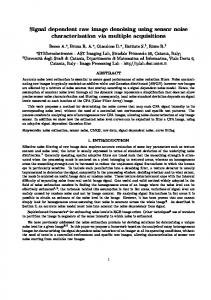
Fig. 2. The effects of subsampling on the filters of a filter bank should be considered when developing a TI scheme.
GN −1 ( z )
H
Fig. 1. A single-level multi-channel filter bank.
coefficients. Below we examine the problem for a general FB. Consider a perfect reconstruction d-dimensional Nchannel FB [8] as illustrated in Fig. 1. We denote M for a d × d sampling matrix. Note that if N = d M , where d M = det( M ) , the FB is critically-sampled and if N > d M , it is oversampled. Suppose we denote the outputs of the analysis filters before downsampling as wi [ n], for 0 ≤ i < N , where n = (n1 , ..., nd )T ∈ Z d . Hence, we have yi [n] = wi [ Mn] . Proposition 1: If one computes all possible shifts of wi [ n] by kc ∈ N ( M ) (0 ≤ c ≤ d M − 1), where d M = det( M ) , and N ( M ) is the set of integer vectors of the form Mt , t ∈ [0,1) d , then the output of the analysis section is translation invariant. Proof: Let us denote the output of channel i for each shift kc as sic (n) ( 0 ≤ i < N , and 0 ≤ c ≤ d M − 1 ), and the set of outputs of channel i as: si [n] = {si 0[ n], ..., si ( d M −1) [ n]} . That is for each channel i, we have d M outputs obtained by shifting wi as sic [ n] = wi [ Mn + kc ] (0 ≤ c ≤ d M − 1, 0 ≤ i < N ) .
Consequently, sic equals the cth polyphase component of wi . Therefore, the output of channel i is a “scrambled” version of wi [ n] . That means, if one shifts the input as x′[ n] = x[n + p ], ( p ∈ Z d ) , one obtains the same shift for wi [ n] , however, si′[n] equals the set of polyphase components of wi′[ n] . Thus, si′[n] = {wi [ Mn + p + kc ]; 0 ≤ c ≤ d M − 1} , which is not simply si [n + p] . It is clear that for a multilevel FB, we can apply the above method at each level for as many inputs as that level has. The above proposed procedure for obtaining a TI scheme is not fast and also it does not directly produce stationary outputs; that is, the outputs need to be unscrambled. Of course this procedure is appropriate in some applications such as adaptive coding, where one needs to find a “best” shift based on a cost function. To avoid the mentioned concerns, below we develop an alternative procedure to obtain the TI scheme. Proposition 2 [5]: In a single-level multidimensional perfect reconstruction FB (see Fig. 1), if we omit the sampling operations, the new TI output, xt , will be a scaled version of xr , i.e. xt = axr , where a = 1/ d M . The redundancy of the resulting TI FB is equal to N. According to Proposition 2, one can simply omit the subsampling operations at a single-level FB scheme to obtain a TI realization of the FB. For a multilevel FB, however, we □
cannot merely omit the subsmapling operations at every level to construct the corresponding TI scheme. Note that at the original FB with subsampling, the input for a level j + 1 is the downsampled version of the output of level j. Therefore, in the nonsubsampled version of the FB, one should change the analysis filters of the level j + 1 in such a way that they operate in the same way as when we have subsampling. The next proposition states how one can construct new filters when one omits the subsampling operations in a multilevel FB, in order to achieve translation invariance. Proposition 3 (generalized algorithme a trous): Assume that we have an L-level multi-channel FB with H i(l ) ( z ) and analysis and synthesis filters (l ) Gi ( z ) (0 ≤ i < N , 1 ≤ l ≤ L) , respectively and sampling matrix M. If one omits the subsampling operations in the FB to obtain the TI scheme, the new analysis and synthesis filters l −1 at a level l , (1 ≤ l ≤ L) are H i(l ) ( z ) = H i ( z M ) and (l ) M l −1 ) , respectively. Gi ( z ) = Gi ( z Proof: Let us prove this proposition through induction. For the first level ( l = 1 ), the proof was given in Proposition 2, that is, the filters remain unchanged. Now suppose l −1 we have the TI filters of H i(l ) ( z ) = H i ( z M ) and (l ) M l −1 ) for level l. Assume that the output of the Gi ( z ) = Gi ( z analysis part at this level is Yi (l ) ( z ) (0 ≤ i < N ) . Now at the next level, l + 1 , we apply a FB using the previous level filters, which are H i(l ) ( z ) and Gi(l ) ( z ) . Since in the original FB, each analysis (synthesis) filter presumes a downsampled (upsampled) version of the output of the last level, as depicted in Fig. 2, the equivalent filters are obtained using the noble identities: H i(l +1) ( z ) = H i(l ) ( z M ) and Gi(l +1) ( z ) = Gi(l ) ( z M ) . l −1 l Hence, H i(l +1) ( z ) = H i ( z ( M ) M ) = H i ( z M ) , and Ml ( l +1) ( M l −1 ) M Gi ( z ) = Gi ( z ) = Gi ( z ) . □
The following corollary generalizes Proposition 3 when the sampling matrices could vary over the different levels. Corollary 1: Suppose that M l (1 ≤ l ≤ L) is the sampling matrix for level l in the filter bank mentioned in Proposition 3. Then the equivalent analysis and synthesis filters for the nonsubsampled filter bank for levels l ≥ 2 (they remain unchanged for the first level) are l −1 l −1 ∏ Mj ∏ Mj H i(l ) ( z ) = H i ( z j =1 ) , and Gi(l ) ( z ) = Gi ( z j =1 ) . Proposition 3 (and its corollary) is indeed an extension of the well-known algorithme a trous [7]. This algorithm was introduced for the wavelet transform where one constructs undecimated or nonsubsampled wavelets. Employing this procedure, one can construct the TI scheme of a filter bank system in a rather straightforward manner.
3. TI CONTOURLET TRANSFORM (TICT)
H ( z)
Since the contourlet transform is realized using two stages of subsampled filter banks, to create a TI contourlet transform (TICT), we should develop the TI schemes for both stages: the LP and DFB, as we explain below.
H
T ( z ) = H ( z ) z k0 − G0 ( z M ) H ( z ) ⋯ z k3 − G3 ( z M ) H ( z ) = ( H ( z ) K 0 ( z ) ⋯ K3 ( z ) ) , T
(
)
T
S ( z ) = G ( z ) z − k0 − G ( z ) H 0 ( z M ) ⋯ z − k3 − G ( z ) H 3 ( z M ) = ( G ( z ) F0 ( z ) ⋯ F3 ( z ) ) .
)
H i ( z ) and Gi ( z ) are the polyphase components of h[ n] and g[ n] in the z-domain, where hi [ n] = h[ Mn − ki ] and gi [ n] = g[ Mn + ki ] (0 ≤ i ≤ 3) , and 0 0 1 1 {ki }0 ≤i ≤3 = , , , , 0 1 0 1 are cosets of M [8] and (⋅)T denotes the transpose of a matrix. To construct a multilevel LP, one can simply iterate the single-level LP on the lowpass channel. And according to Section 2, the multilevel TI scheme of the LP is constructed by suppressing all subsampling operations and modifying the filters at level l as, T
(l )
(
l −1
l −1
l −1
l −1
l −1
( z ) = H ( z M ) K 0 ( z M ) ⋯ K3 ( z M )
and
(
l −1
)
T
,
)
S (l ) ( z ) = G ( z M ) F0 ( z M ) ⋯ F3 ( z M ) , l −1
l −1
Y1 ( z )
M
G(z)
M
F1 ( z )
H H
M
Y3 ( z )
M
H T ( z)
Do and Vetterli proposed a new reconstruction scheme for the LP based on the frame reconstruction [2]. They also expressed the LP in the polyphase domain [8] in the form of an oversampled FB that is a suitable form for realizing the TILP. Fig. 3 shows the resulting 2-D FB assuming that the lowpass and highpass filters in the LP are H and G [2][5]. Here M = diag(2, 2) is the sampling matrix,
and
M
Y0 ( z )
H K3 ( z )
3.1. TI Laplacian Pyramids (TILP)
(
K0 ( z )
x
M
xr
F3 ( z )
H S ( z)
Fig. 3. One-level 2-D LP in the form of an oversampled FB. ˆ
Si(l ) , where diag(2lˆ −1 ,2), if 0 ≤ i < 2lˆ −1 ˆ Si(l ) = . ˆ ˆ ˆ diag(2,2l −1 ), if 2l −1 ≤ i < 2l Since this FB scheme is the equivalent iterated DFB system for lˆ levels, to construct the TI scheme, it is sufficient to suppress the subsampling operations and multiply the reconstructed signal by a scaling factor, which is ˆ ˆ 1/ det( Si(l ) ) = 2−l . Therefore, the redundancy of such scheme ˆ is equal to the number of directions 2l .
3.3. TI and Semi-TI Contourlet Transforms The TI contourlet transform (TICT) is constructed using the TILP and TIDFB. In fact, we employ a similar structure as the one we used in the contourlet transform; however, in developing the TICT, since every level of the TILP has four highpass subbands, we are required to apply the TIDFB to each one of these subbands. To preserve the anisotropy scaling law of width = length 2 , we apply a TIDFB with a desired maximum number of directional levels to the four finest subbands of the TILP, where we are at level one, then as we decrease the radial resolution of the TILP at higher levels, we decrease the directional levels at every other TILP level. Proposition 4: Assume that a TILP has L levels and we apply an lˆ -level (1 ≤ i ≤ L ) TIDFB to the four detail i
subbands of level i of the TILP. Then the redundancy of the
l −1
where z M = ( z12 , z22 ) , which implies that we upsample the corresponding filters in both the row and column directions with 2l −1 . Note also that we should scale the signal after each synthesis bank by ¼. In the TILP scheme, since there are four detail channels at each level, the redundancy of this scheme is 4 L + 1 , when an L-level scheme is employed.
3.2. TI Directional Filter Banks (TIDFB) ˆ
In an lˆ -level DFB, we decompose the frequency space to 2l wedge-shaped partitions. It can be expressed by an overall ˆ ˆ FB having 2l analysis and 2l synthesis filters, ˆ ˆ ˆ H i(l ) and Gi(l ) ( 0 ≤ i < 2l ), and the overall sampling matrices
constructed TICT is 4 L∑ i =1 2li + 1 . L
ˆ
Proof: The proof is straightforward noting that the TILP has four detail subbands at each level and the ˆ redundancy of an lˆi -level TIDFB is 2li . □
Since the redundancy of the TIDFB increases exponentially as the number of directional levels is raised, we construct another variety of contourlets. This construction is realized through applying the critically-sampled DFB to the TILP in much the same way we constructed the TICT. The only difference is that we do not use the TI version of the DFB and thus, this realization is indeed non-TI; so, we call it semi-TI contourlet transform (STICT). The redundancy of this scheme is the same as the redundancy of the TILP, that is 4L + 1 .
TABLE I PSNR VALUES OF THE DENOISING EXPERIMENTS WHEN Image WT1 CT2 TIWT3 STICT4 Barbara 25.70 26.31 28.19 29.42 Boats 27.14 26.83 29.68 29.57 Fingerprint 26.21 26.05 28.66 28.45 GoldHill 26.87 26.66 29.08 28.95 Mandrill 22.98 22.66 25.12 24.87 Peppers 28.41 27.69 30.90 30.54 1
4
2
5
Wavlet Transform Contourlet Transform 3 TI Wavelet Transform
40
50 σ
60
70
PSNR (dB)
PSNR (dB)
Fig. 5. Denoising results of the Barbara image at σ = 20 using different schemes (from left to right, top to bottom): TIWT, CT, STICT, TICT.
PSNR values for the Peppers image
WT TIWT CT STICT TICT
30
TICT5 30.06 30.05 28.74 29.36 25.36 31.06
Semi-TI Contourlet Transform TI Contourlet Transform
PSNR values for the Barbara image 31 30 29 28 27 26 25 24 23 22 21 20 20
σ = 20
80
32 31 30 29 28 27 26 25 24 23 22 21 20 20
WT TIWT CT STICT TICT
30
40
50 σ
60
70
80
Fig. 4. PSNR results of the image denoising experiments for the Barbara and Peppers images.
4. IMAGE DENOISING The contourlet transform has been shown to be a better alternative choice than wavelets for image denoising [3]-[5]. In [4], a cycle-spinning algorithm is employed to improve the denoising performance of contourlets. Although it is equivalent to a TI denoising if all of the possible shifts of the input image are used, the computational complexity of this procedure is too high, which consequently makes this algorithm almost prohibitive for rather large-size images. In contrast, the proposed method in this paper achieves TICT with a feasible load of computation. To evaluate the proposed schemes, we performed several experiments on a variety of images all of size 512 × 512 . We used biorthogonal Daubechies 9/7 wavelets for comparison. A TI wavelet transform (TIWT) is implemented using the approach mentioned in Section 2. Hence, a TIWT with L levels has a redundancy of 3L + 1 . For the LP stage of contourlets we also used the same biorthogonal filters and applied 6 levels of decomposition. The images are contaminated by a zero-mean Gaussian noise with a standard deviation of σ , ranging from 20 to 80. Since for TI denoising, hard-thresholding usually yields better results than soft-thresholding, we used hard-thresholding with a fixed threshold value equal to τ = 3σ [6]. Table I shows the PSNR results of the denoising experiments when σ = 20 . We see that the TICT yields superior results in all cases. In particular, for the Barbara image, there is a gain of over 1.8 dB in comparison to the PSNR value achieved by the TIWT. Furthermore, the PSNR values attained by the suboptimal method of STICT are up to 0.6 dB less than those of the TICT. The PSNR vs. standard deviation curves for the images Barbara and Peppers are provided in Fig. 4. As seen, the TICT approach yields better results at most cases. Fig. 5
shows the denoised results of the Barbara image at σ = 20 . It is clear that the TICT denoising scheme is capable of further retaining edges and fine details when compared with the TIWT scheme. Remarkably, the CT scheme introduces a significant amount of artifacts and since TI denoising considerably reduces these artifacts, the TICT denoising approach yields better results at most cases (Fig. 4).
5. CONCLUSIONS In this work we developed a procedure to obtain a TI version of a general multi-channel multidimensional subsampled FB, where we proposed a generalized algorithme a trous, and then applied the derived approach to the contourlet transform. In addition to the proposed TI contourlets, we introduced semi-TI contourlets, which is less redundant than the TICT. Furthermore, we employed our proposed schemes in conjunction with the TIWT to image denoising. Our simulation results indicate the potential of the TICT and STICT for image denoising, where one can achieve better visual and PSNR performance at most cases when compared with the TIWT.
6. REFERENCES [1] R. R. Coifman and D. L. Donoho, “Translation Invariant Denoising,” in Wavelets and Statistics, Springer Lecture Notes in Statistics 103, New York, Springer-Verlag, pp. 125-150, 1995. [2] M. N. Do and M. Vetterli, “Framing Pyramids,” IEEE Trans on Signal Processing, vol. 51, no. 9, pp. 2329-2342, Sep. 2003. [3] M. N. Do and M. Vetterli, “The Contourlet Transform: An Efficient Directional Multiresolution Image Representation,” to appear in IEEE Trans. on Image Processing, 2004. [4] R. Eslami and H. Radha, “The Contourlet Transform for Image De-noising Using Cycle Spinning,” in Asilomar Conf. on Signals, Systems, and Computers, pp. 1982-1986, Pacific Grove, Nov. 2003. [5] R. Eslami and H. Radha, “Translation-Invariant Contourlet Transform and Its Application to Image Denoising,” submitted to IEEE Trans. on Image Processing, 2004. [6] M S. Mallat, A Wavelet Tour of Signal Processing. Academic Press, 2nd Ed., 1998. [7] M. J. Shensa, “The Discrete Wavelet Transform: Wedding the a Trous and Mallat Algorithms,” IEEE Trans. on Signal Processing, vol. 40, no. 10, pp. 2464-2482, Oct. 1992. [8] P. P. Vaidyanathan, Multirate Systems and Filter Banks. Prentice Hall, 1993.