2009 Fifth International Conference on Image and Graphics
Image Denoising Via Sparse and Redundant Representations Over Learned Dictionaries in Wavelet Domain Huibin Li Feng Liu Department of Information and Computing Science, School of Science Xi’an Jiaotong University, Xi’an, 710049, China
[email protected]
Abstract
[email protected]
transform, the multi-scale structure of image can been captured very easily. At the same time, the assumption of sparse representations of wavelet coefficients over redundant dictionary or even orthogonal basis can been achieved very naturally. In this natural way, the prior-learning on the corrupted image is transferred to the wavelet coefficients of it. And the adaptive dictionaries have been learned in wavelet domain. It means image denoising in the framework of sparse representations in wavelet domain. As a first attempt to this fusion, single-scale wavelet decomposition technology is used. Experiments show that this new method performs a better visual effect and higher values of PSNR than K-SVD method[2] when we are concerning strong white Gaussian noise.
This paper proposes a novel hybrid image denoising method based on wavelet transform and sparse and redundant representations model which is called signal-scale wavelet K-SVD algorithm (SWK-SVD). In wavelet domain, mutiscale features of images and sparse prior of wavelet coefficients are achieved in a natural way. This gives us the motivation to build sparse representations in wavelet domain. Using K-SVD algorithm, we obtain adaptive and over-complete dictionaries by learning on image approximation and high-frequency wavelet coefficients respectively. This leads to a state-of-art denoising performance both in PSNR and visual effects with strong noise.
2. The K-SVD denoising method 1. Introduction
2.1. Sparse and redundant representations model of signal
Recently, sparse and redundant representations model is applied to image denoising and has drawn a lot of researchers’ attention. In [1], the K-SVD algorithm was proposed for learning a single-scale adaptive dictionary for sparse representation of gray-scale image patches. Inspired by the idea of prior-learning on the corrupted image, the KSVD algorithm was used to remove white Gaussian noise, leading to a very competitive method [2,3]. Then, this work was extended to various applications such as color image denoising[4], demosaicing, inpainting, and video denoising [7], getting state-of-the-art performances. More recently, multi-scale K-SVD method has been proposed, which combine sparsity and multi-scale techniques in a learning fashion [7]. Considering these two concepts have been both wildly applied and studied independently in image processing, this paper is also built on the concepts of multi-scale and sparsity. But different from using a quadtree decomposition model [7], wavelet transform, as a powerful multi-scaled analysis tool, which has made a tremendous success in image denoising [6], is applied in this paper. By using wavelet 978-0-7695-3883-9/09 $26.00 © 2009 IEEE DOI 10.1109/ICIG.2009.101
Given a signal y ∈ Rn and a over-completed dictionary D = [d1, d2 , · · · , dk ] ∈ Rn×k (n ≪ k), where di is called atom. The sparse and redundant representations model of signal is equivalent to the following problem: (P0 ) : min ∥α∥0 s. t. y = Dα. α
(1)
here ∥α∥0 = # {i : αi ̸= 0} is called l0 norm. It defines the sparsity measurement of the vector α. Generally speaking, (P0 ) is a large combinatorial optimization problem. So researchers always try to find a approximate solution like Orthogonal Matching Pursuit(OMP) algorithm[8].
2.2. Sparse and redundant representations model for image denoising We address the classical image denoising problem: a clear image x is corrupted by an additive zero-mean white and homogeneous Gaussian noise z, with standard deviation σ and ∥z∥2 ≤ ε, and the observed image y is generated. 754
Hence,
the Lagrange form of it is: y = x + z.
2
α ˆ ij = arg min ∥LW xij − Dαij ∥2 + µij ∥αij ∥0 .
(2)
αij
Assume x ∈ R has sparse representation over redundant dictionary, modifying (P0 ), we get the denoising model as follows:
(6)
n
2
(P0,δ ) : α ˆ = arg min ∥α∥0 s.t. ∥y − Dα∥2 ≤ δ. α
By maximum a posteriori (MAP) estimation, denoising of LW y is equivalent to the energy minimization problem: 2
{ˆ αij , LW x ˆ} = arg min λ ∥LW x − LW y∥2
(3)
Here δ = δ(ε). And we get the restoration of image x ˆ = Dα ˆ.
+
αij ,LW x
µij ∥αij ∥0 +
ij
2.3. The K-SVD image denoising method
∑
2
∥Rij LW x − Dαij ∥2 .
(7)
ij
In this expression, the first term is the log-likelihood between LW x and LW y, and λ depends on 2 ∥LW x − LW y∥2 ≤ Const · σ 2 . The second and the third terms are the sparse prior of wavelet coefficients. When D is known, we can solve (7) by two steps.√First, let √ LW x 2= LW y, thus (7) is equivalent to solve ( N − n + 1) problems of (6) which can be solved by OMP. This step is called sparse coding. Second, when getting α ˆ ij for all (ij) locations, fix them and turn to update LW x. Returning to (7), we need to solve:
The key point for solving problem (P0,δ ) is to find the suitable redundant dictionary, for this reason the K-SVD algorithm [1] is proposed. The basic idea is: when the training signal and the initial dictionary are given, then the priorlearning idea is used. It learns a dictionary that yields sparse representations for the training signal. The algorithm alternates a sparse coding step based on a Orthogonal Matching Pursuit (OMP) and a dictionary updating step based on a simple Singular Value Decomposition (SVD). In particular, if K = 1 we get the well known K-means algorithm. The reader can refer to [1, 2] for some details.
2
LW x ˆ = arg min λ ∥LW x − LW y∥2 LW x ∑ 2 + ∥Rij LW x − Dα ˆ ij ∥2 .
3. Hybrid denoising method using Wavelet and K-SVD
(8)
ij
This is a simple quadratic programming that has a closedform solution:
√ √ In (2), we assume clear image x of size N × N pixels, and then use two-dimension discrete single-scale wavelet transform by suitable wavelet basis√on the observed image √ y. It gets four little patches of size ( N /2) × ( N /2) pixels, they are the image approximation coefficients and horizontal, vertical and diagonal directions of the three wavelet coefficients, noted by LW y, HW y, V W y and DW y respectively. First, we estimate LW x. According to (2) and the property of wavelet transform, we have: LW y = LW x + LW z.
∑
LW x ˆ = (λI +
∑
T Rij Rij )−1 (λLW y +
ij
∑
T Rij Dα ˆ ij ). (9)
ij
This expression says the averaging of the denoised patches and is called patches averaging step. Given the updated, we can repeat the sparse coding stage, working on the already denoised patches. Once this is done, a new averaging should be calculated, and so on, and so forth. Finally, the satisfying α ˆ ij and LW x ˆ are obtained. In practice, the dictionary D is unknown and we can get it by learning which is same to [1]. After fusion dictionary learning in (7), we get the denoising model as follows: { } 2 ˆ LW x α ˆ ij , D, ˆ = arg min λ ∥LW x − LW y∥2
(4)
where LW x and LW z are the wavelet transform of x and z respectively. Just like K-SVD algorithm learning dictionary on small image patches, note √ each small √ patch LW xij = Rij LW x ∈ Rn×1 of size ( n) × ( n) (or stacking its columns as size of n × 1) in every location (i,j) of LW x. where Rij ∈ Rn×(N/4) is a matrix that extracts the √ (ij) block √size of n×1 pixels from LW x. For its size of ( N /2) × ( N√/2), consider all position (ij) and all small √ patches of size n × n with overlaps, it √ is easy to know √ the summation over i, j includes ( N /2 − n + 1)2 items. When redundant dictionary D ∈ Rn×k is given, According to the prior of wavelet coefficients, every patch has a sparse representation with bounded error, we get:
+
∑ ij
αij ,D,LW x
µij ∥αij ∥0 +
∑
2
∥Rij LW x − Dαij ∥2 . (10)
ij
In this paper, K-SVD algorithm is used to learn and update initial redundant DCT dictionary, and LW yij is the training set. As so far, we can solve (10) as follows: a) Given the initial dictionary D and let LW x = LW y, then ˆ uscompute α ˆ ij by (5); b) update initial dictionary D to D ˆ and ing K-SVD; c) compute LW x ˆ by (9). Finally, let D
2
α ˆ ij = arg min ∥αij ∥0 s.t. ∥LW xij − Dαij ∥2 ≤ (Cσ)2(5) αij
755
Table 1. Summary of the denoising PSNR(dB) results. In each cell, two denoising results are reported, in each such set we highlight the better result. Left: K-SVD method [2]. Right: SWK-SVD method. σ/PSNR 15/24.61 20/22.11 25/20.17 50/14.15 60/12.58 70/11.23 80/10.08 90/9.09 100/8.13
Barb 32.37 31.66 30.83 30.06 29.60 28.96 25.47 25.72 24.23 24.78 23.32 24.02 22.67 23.40 22.19 22.71 21.89 22.22
Boats 31.73 31.21 30.36 29.91 29.28 28.92 25.95 25.96 24.80 24.95 24.26 24.33 23.65 23.69 23.25 23.36 22.81 22.82
{ˆ αij (l)}(i,j)∈wl = σ1 · v1T . Updating all dl , we get updated ˆ = [dˆ1 , dˆ2 , · · · , dˆk ]. dictionary D ˆ in (9), and then compute LW x 2.4: Set D = D ˆ. 2.5: Set p = p + 1. If p = J, turn to Step 3. If not, set ˆ in (10). Turn to step 2.2. Step LW x=LW x ˆ and D = D 3: Similar to LW y, implement step 2 to HW y, V W y and DW y respectively and get HW x ˆ, V W x ˆ and DW x ˆ. Step 4: Use inverse wavelet transform on LW x ˆ, HW x ˆ, V Wx ˆ and DW x ˆ, getting the denoised image x ˆ.
House 34.32 33.57 33.20 32.36 32.15 31.51 27.95 28.14 26.68 27.22 25.67 26.31 24.90 25.64 24.19 24.73 23.71 24.11
4. Numerical experiment In this section, we demonstrate the results achieved by applying our approach and K-SVD method under various noise levels. The tested images, as also the parameters in our algorithm are all the same ones as those used in the denoising experiments reported in [2]. In order to enable a fair comparison, db4 wavelet basis is used in our approach. Every result reported is an average over 5 experiments, having different realizations of the noise. As can be seen from Table I, the results of this two methods are very close to each other in general. For the low noise power less than σ = 50 , our approach achieves weaker results. But for higher noise power equal to or bigger than σ = 50, our approach achieves better results than K-SVD method. Figure 1 shows the results of the K-SVD method and the proposed approach for image “House” with noise standard deviation of 25. As can be seen from Figure 1, although the PSNR of denoised image by SWK-SVD(31.51 dB) is small corresponding to K-SVD(32.15 dB), the denoised image by
LW x ˆ are the initial D and LW x, then repeat the above process until we satisfied with the result. As for LW y, do the same process on HW y, V W y and DW y, getting the denoised image HW x ˆ, V W x ˆ and DW x ˆ. As so far, we have finished the denoising process in wavelet domain, and the inverse wavelet transform is used to get the restoration image x ˆ. Because only single-scale wavelet transform is used in our algorithm, we name our method as signal-scale wavelet K-SVD (SWK-SVD). The detailed steps of this algorithm can be given below: Step 1: Choose suitable wavelet basis, use twodimension discrete single-scale wavelet transform on the observed image y and get LW y, HW y, V W y and DW y. Step 2: Do the following operation for LW y. 2.1: Choose the parameters λ-Lagrange, noise gain-C, number of atoms-k, size of patches-n and number of training iterations-J. Set LW x ˆ=LW y, D = redundant DCT dictionary. Set P = 0 as the counter of loop. 2.2: Use OMP to compute coefficients α ˆ ij ∈ Rk×1 for each patch by solving (5). 2.3: Update the dictionary. For each column l = 1, 2, · · · k in D, as a atom of dictionary, update it by the following steps: • Find the set of patches that use this atom, ωl = {[i, j]|ˆ αij (l) ̸= 0}. • For each index [i, j] ∈ ωl , compute its representation error: ∑ elij = Rij LW x − dm α ˆ ij (m). m̸=l
• set El as the error matrix whose columns are (elij )[i,j]∈ωl ∈ Rn×|ωl | . • Apply SVD decomposition El = U ∆V T , where U = (u1 , u2 , · · · , un ), ∆ = diag(σ1 , σ2 , · · · σn ), σ1 ≥ σ2 ≥ · · · ≥ σr > σr+1 = · · · = σn = 0 are singular values and V = (v1 , v2 , · · · , v|wl | ). Set dˆl = u1 and
Figure 1. Example of the denoising results for the image “House” with σ = 25, from left to right and top to bottom: the original image, the noisy image(20.17 dB), Denoised iamge by K-SVD(32.15 dB), Denoised image by SWK-SVD method(31.51 dB).
756
image edges and flat areas are blurred. While the denoised image by SWK-SVD is more clear and smooth in whole image and have a better visual effect. Figure 3 and Figure 4 shows the dictionaries learned on the noisy image respectively by K-SVD and SWK-SVD under the noise levels of σ = 25 and σ = 50. It shows that the dictionaries learned by SWK-SVD method was divided to four parts. They are achieved by learned on image approximation and three high-frequency wavelet coefficients respectively in single-scale wavelet domain.
5. Conclusion and Discussion This work has extended the method using the sparse and redundant representations denoising model based on KSVD algorithm to wavelet domain.Demonstrated by lots of experiments, we show that the proposed method achieves better results on PSNR and visual effect than K-SVD at high noise levels. But at low noise levels, our method just gets better results on visual effect and a little lower PSNR than K-SVD. The reasons why our proposed method get these results certainly contribute to the wavelet we use. But the intrinsic reasons is not clear for us. Recently the cross-andbouquet model[9] has successfully explained the error correction ability of l1 minimization in recognition, and the authors said that ” the striking discriminative power of the sparse representation still lacks rigorous mathematical justification. To the best of our knowledge, this remains a wide open topic for future investigation[9].” This paper is an initial attempt to build sparse representations model for image denoising in single-scale wavelet domain. We are mainly interested in combining sparse representations with multi-scale wavelet decomposition technology and various wavelet shrinkage algorithms to compete with [7] in our further work. And also concerned with choosing the right wavelet basis and estimating the noise gain-C in wavelet domain, and etc.
Figure 2. Example of the denoising results for the image “House” with σ = 50, from left to right and top to bottom: the original image, the noisy image(14.15 dB), Denoised iamge by K-SVD(27.95 dB), Denoised image by SWK-SVD method(28.14 dB).
Figure 3. Dictionaries learned on the noisy image“House” with σ = 25, learned by K-SVD method(left) and by SWK-SVD method(right).
References [1] M.Aharon, M Elad and A.M.Bruckstein. The k-svd: An algorithm for designing of overcomplete dictionaries for sparse representations. IEEE Trans. Signal Process, 54(11):4311– 4322, November 2006.
Figure 4. Dictionaries learned on the noisy image“House” with σ = 50, learned by K-SVD method(left) and by SWK-SVD method(right).
[2] M.Elad and M.Aharon. Image denoising via sparse and redundant representations over learned dictionaries. IEEE Trans.Image Process, 15(12):3736–3745, December 2008.
SWK-SVD method seems more clear and smooth than the denoised image by K-SVD method. Figure 2 shows the results of the K-SVD method and the proposed approach for image “House” with noise standard deviation of 50. As can be seen from Figure 2, the denoised image by K-SVD have slight fluctuations and the
[3] M.Elad and M.Aharon. Image denoising via learned dictionaries and sparse representation. CVPR, (1):895–900, 2006. [4] M. J.Mairal and G.Sapiro. Sparse representation for color image restoration. IEEE Trans.Image Process, 17(1):53–69, January 2008.
757
[5] M.Protter and M.Elad. Image sequence denoising via sparse and redundant representations. IEEE Trans.Image Process, 18(1):27–35, December 2009. [6] D. L. Donoho. De-noising by soft-thresholding. IEEE Trans. on Information Theory, 41(3):613–627, May 1995. [7] M. J.Mairal and G.Sapiro. Learning multiscale sparse representations for image and video restoration. SIMA,Multiscale Model. Simul, 7(1):214–241, April 2008. [8] R. R. Y.C. Pati and P. Krishnaprasad. Orthogonal matching pursuit: recursive function approximation with applications to wavelet decomposition. 27th Annu. Asilomar Conf. Signals, Systems, and Computers, 43(1):40–44, 1993. [9] J.Wright, Yi Ma and J.Mairal etc. Sparse Representation For Computer Vision and Pattern Recognition. Proceedings of the IEEE Special Issue on: Applications of Sparse Representation and Compressive Sensing, 1-10, March, 2009.
758