Image Features for Visual Teach-and-Repeat Navigation in Changing

Image Features for Visual Teach-and-Repeat Navigation in Changing Environments Tom´asˇ Krajn´ıka , Pablo Crist´oforisb , Keerthy Kusumama , Peer Neubertc , Tom Ducketta a Lincoln

Centre for Autonomous Systems, University of Lincoln, UK of Robotics and Embedded Systems, University of Buenos Aires, Argentina c Dept. of Electrical Engineering and Information Technology, Technische Universit¨ at Chemnitz, Germany b Laboratory

Abstract We present an evaluation of standard image features in the context of long-term visual teach-and-repeat navigation of mobile robots, where the environment exhibits significant changes in appearance caused by seasonal weather variations and daily illumination changes. We argue that for long-term autonomous navigation, the viewpoint-, scaleand rotation- invariance of the standard feature extractors is less important than their robustness to the mid- and longterm environment appearance changes. Therefore, we focus our evaluation on the robustness of image registration to variable lighting and naturally-occurring seasonal changes. We combine detection and description components of different image extractors and evaluate their performance on five datasets collected by mobile vehicles in three different outdoor environments over the course of one year. Moreover, we propose a trainable feature descriptor based on a combination of evolutionary algorithms and Binary Robust Independent Elementary Features, which we call GRIEF (Generated BRIEF). In terms of robustness to seasonal changes, the most promising results were achieved by the SpG/CNN and the STAR/GRIEF feature, which was slightly less robust, but faster to calculate. Keywords: visual navigation, mobile robotics, long-term autonomy

1. Introduction Cameras are becoming a de-facto standard in sensory equipment for mobile robotic systems including field robots. While being affordable, small and light, they can provide high resolution data in real time and virtually unlimited measurement ranges. Moreover, they are passive and do not pose any interference problems even when deployed in the same environment in large numbers. Most importantly, the computational requirements of most machine vision techniques are no longer a significant issue due to the availability of powerful computational hardware. Hence, on-board cameras are often used as the primary sensors to gather information about the robot’s surroundings. Many visual robot navigation and visual SLAM methods rely on local image features [1] that allow to create quantitatively sparse, but information-rich image

descriptions. These methods consist of a detection and a description step, which extract salient points from the captured images and describe the local neighborhood of the detected points. Local features are meant to be detected repeatedly in a sequence of images and matched using their descriptors, despite variations in the viewpoint or illumination. Regarding the quality of feature extractors, a key paper of Mikolajczyk and Schmid [2] introduced a methodology for evaluation of feature invariance to image scale, rotation, exposure and camera viewpoint changes. Mukherjee et al. [3] evaluated a wide range of image feature detectors and descriptors, confirming the superior performance of the SIFT algorithm [4]. Other comparisons were aimed at the quality of features for visual odometry [5] or visual Simultaneous Localization and Mapping (SLAM) [6]. Unlike the aforementioned works, we focus our evaluation on navigational aspects, especially to achieve long-term autonomy under seasonal changes.

Email addresses: [email protected] (Tom´asˇ Krajn´ık), [email protected] (Pablo Crist´oforis), [email protected] (Keerthy Kusumam), [email protected] (Peer Neubert), [email protected] (Tom Duckett)

Although the problem of long-term autonomy in changing environments has received considerable attention during the last few years [7], the main efforts were aimed at place recognition [8] and metric local-

Accepted for publication in Robotics and Autonomous Systems

November 26, 2016

tor (SpG) [18]. We also propose a trainable feature descriptor based on evolutionary methods and binary comparison tests and show that this algorithm, called GRIEF (Generated BRIEF), and the SpG/CNN feature outperform the engineered image feature extractors in their ability to deal with naturally-occurring seasonal changes and lighting variations [19]. This adaptive approach allows to automatically generate visual feature descriptors that are more robust to environment changes than standard hand-designed features. The work presented here broadens our previouslypublished analysis [19] by including new datasets (‘Nordland’ [18]), image features (SpG/CNN) and feature training schemes. In particular, we separate the influence of the detector and descriptor phases on the robustness of the feature extractors to appearance changes and demonstrate that combination of detection and description phases of different features can result in feature extractors that are more robust to seasonal variations. Moreover, we perform a comparative analysis of training schemes, leading to computationally-efficient image features that can deal with naturally-occurring environment changes. We apply our evaluation on a new dataset, which became available only recently [20]. Finally, we provide the aforementioned benchmarking framework and the GRIEF training method as a documented, open-source software package [21].

ization [9]. Unlike these works, we focus on the image processing aspect of long-term navigation in the context of teach-and-repeat systems [10], where a key issue is robust estimation of the robot heading [11, 12].

Figure 1: Examples of tentative matches of the GRIEF image features across seasonal changes.

Let us consider a scenario where a mobile robot navigates along a previously mapped path using vision as the main sensory modality. Typically, the robot would keep close to the previously learned path and it will not be necessary to use image features that are highly invariant to significant viewpoint changes. One can also assume that the surface in the path vicinity will be locally planar, which means that rotational invariance of the image features is not important either. On the other hand, the appearance of outdoor environments changes over time due to illumination variations, weather conditions and seasonal factors [13]. After some time, the environment appearance might differ significantly from its pre-recorded map, making long-term map-based visual navigation a difficult problem. We hypothesize that for the purpose of teach-andrepeat visual navigation, the invariance of the image features to scale, rotation and viewpoint change is less important than their robustness to seasonal and illumination variations. These considerations motivate us to analyze available feature detector and descriptor algorithms in terms of their long-term performance in autonomous navigation based on a teach-and-repeat principle, e.g., as used in [10, 11, 12, 14]. In this work, we present an image feature evaluation methodology which is tailored for teach-and-repeat navigation in long-term scenarios. We show the results achieved using combinations of open-source feature detectors and descriptors such as BRIEF [15], (root)SIFT [4], ORB [16] and BRISK [17]. Moreover, we evaluate a feature based on a Convolutional Neural Network (CNN) descriptor and a Superpixel Grid detec-

2. Visual navigation in changing environments The problem of vision-based localization and mapping has received considerable attention during the last decades and nowadays robots can create create precise maps of very large environments and use these maps to determine their position with high accuracy. Localization itself was typically studied in the context of Simultaneous Localization and Mapping (SLAM), where the position estimate was based on a map that was built on-the-fly and, therefore, the effects of environment changes had only marginal importance. However, as the operation time of the robots increased, they have to face the problem that cameras are inherently passive and their perception of the environment is heavily influenced by illumination factors which tend to change throughout the day. This issue motivated research into methods that are able to suppress the effects of naturally-changing outdoor illumination. One of the popular methods [22] calculates illumination-invariant images by exploiting the fact that the wavelength distribution of the main outdoor illuminant, the sun, is known. This method improves 2

robot localization and navigation in outdoor environments [23, 24, 25, 26], but can cope only with changes caused by varying outdoor illumination during the day. A recent work by Mount and Milford also reported that low-light cameras [27] can provide images that allow reliable day/night localisation. However, appearance changes are not caused just by varying illumination, but also by the fact that the environment itself changes over time. Valgren and Lilienthal [13] addressed the question of environment change in vision-based localization by studying the robustness of SIFT and SURF image features to seasonal variations. The paper indicated that as robots are gradually becoming able to operate for longer and longer time periods, their navigation systems will have to address the fact that environment itself, not only the illumination, is subject to constant, albeit typically slow, changes. Some approaches aimed at solving the problem by using long-term observations to identify which environment features are more stable. Dayoub and Duckett [28] presented a method that continuously adapts the environment model by identifying stable image features and forgetting the unstable ones. Rosen et al. [29] used Bayesian-based survivability analysis to predict which features will still be visible after some time and which features will disappear. Carlevaris et al. [30] proposed to learn visual features that are robust to the appearance changes and showed that the learned features outperform the SIFT and SURF feature extractors. Lowry et al. [31] used principal component analysis to determine which aspects of a given location appearance are influenced by seasonal factors and presented a method that can calculate ‘condition-invariant’ images. Cieslewski et al. [32] show that a sparse 3D environment description obtained through structure-from-motion approaches is robust to seasonal changes as well. Some works use the long-term observations to build models that can predict the appearance of a given location at a particular time. Lowry et al. [33] applied linear regression techniques directly to the image space in order to predict the visual appearance of different locations in various conditions. S¨underhauf and Neubert [34, 35] mined a dictionary of superpixel-based visual-terms from long-term data and used this dictionary to translate between the appearance of given locations across seasons. Krajnik et al. [36] used Fourier analysis to identify the cyclical changes of the environment states and showed that predicting these states for a particular time improves long-term localization [37]. Another group of approaches proposes to use multiple, condition-dependent representations of the environment. For example, Churchill and Newman [9] clus-

tered different observations of the same place to form “experiences” that characterize the place appearance in particular conditions. McManus et al. [38] used dead reckoning to predict which place the vehicle is close to, loaded a bank of Support Vector Machine classifiers associated with that place and used these to obtain a metric pose estimate. Krajnik et al. [39] proposed to maintain maps gathered over an entire year and select the most relevant map based on its mutual information with the current observation. Methods based on deep learning, which has had a big impact on the field of computer vision, were also applied to the problem of persistent navigation. Neubert and Protzel [18] showed that image descriptors based on Convolutional Neural Networks (CNN) outperformed the best holistic place recognition methods while being able to handle large viewpoint changes. S¨underhauf et al. [8, 40] also demonstrated impressive results with CNN-based methods. However, the recent outcome of the Visual Place Recognition in Changing Environments, or VPRiCE Challenge [41] indicated that novel, yet classic-feature-based approaches, such as [42] performed better than the CNN-based methods. Most of the aforementioned approaches were aimed at place recognition [7] and metric localization [9]. Unlike these works, we focus on the image processing aspect of long-term navigation in the context of teach-andrepeat systems [10], where a key issue is robust estimation of the robot heading [11, 12]. 3. Local image feature extractors Local image features provide a sparse, but distinctive representation of images so that these can be retrieved, matched or registered efficiently. The feature extraction process consists of two successive phases: feature detection and feature description. The detector identifies a salient area in an image, e.g. a corner, blob or edge, which is treated as a keypoint. The descriptor creates a vector that characterizes the neighborhood of the detected keypoint, typically in a scale-affine invariant way. Typical descriptors capture various properties of the image region like texture, edges, intensity gradients, etc. The features are meant to be repeatably extracted from different images of the same scene even under conditions of unstable illumination or changing viewpoints. In this paper, we evaluate several image feature extraction algorithms for the purpose of long-term robot navigation. Most of these algorithms are included in the Open Source Computer Vision (OpenCV) software library (version 2.4.3), which was used to generate the results presented in this paper. 3

are first marked as bright, neutral or dark depending on their brightness relative to the central pixel. The central pixel is considered as a keypoint if the circle contains a contiguous sequence of at least n bright or dark pixels (a typical value of n is 12). In order to quickly reject candidate edges, the detector uses an iterative scheme to sample the circle’s pixels. For example, the first two examined pixels are the top and bottom one - if they do not have the same brightness, a contiguous sequence of 12 pixels cannot exist and the candidate edge is rejected. This fast rejection scheme causes the FAST detector to be computationally efficient.

3.1. Feature Detectors 3.1.1. LoG/DoG (SIFT) The SIFT feature [4] uses a Difference-of-Gaussians detector to find scale-invariant keypoint locations. The feature detection process first generates a scale space of the image by convolving it with Gaussian kernels of different sizes. The DoG detector then searches for local extrema in the images obtained by the difference of two adjacent scales in the Gaussian image pyramid. This gives an approximation of the Laplacian of Gaussian (LoG) function where local extrema correspond to the locations of blob-like structures. A local extremum is found by comparing the DoG values of each point with its 8 pixel neighbourhood and 9 other neighbours in the two adjacent scale levels. This type of keypoint localization allows to detect blobs at multiple scales, resulting in scale invariance of the features. To achieve rotation invariance, SIFT assigns a dominant orientation to the detected keypoint obtained by binning the gradient orientations of its neighborhood pixels.

3.1.5. Oriented FAST and Rotated BRIEF - ORB The ORB feature extractor combines a FAST detector with an orientation component (called oFAST) [16]. The keypoints are identified by the FAST detector and ordered by the Harris corner measure, then the best N keypoints are chosen. The original FAST detector is not scale invariant, hence the ORB detector uses a scale space to identify interest points. Then, the orientation of the feature is calculated using the intensity centroid. The direction of the vector between the intensity centroid and the corner’s centre gives the orientation of the point.

3.1.2. Hessian-Laplace Region (SURF) The Hessian keypoint detector finds interest points that vary in the two orthogonal directions [43]. It computes the second derivatives for each image location and finds the points for which the determinant of the Hessian matrix is maximal. The Hessian-Laplace detector combines the Hessian detector that returns corner-like structures along with a LoG detector. The Hessian detector returns interest points at each scale in the scale space and the Laplacian of Gaussian (LoG) detector searches for the extremum on these interest locations. The SURF detection scheme speeds up the process by approximating the Gaussian scale pyramid using box filters.

3.1.6. Binary Robust Invariant Scalable Keypoints The BRISK feature detector is scale and rotation invariant [17]. To identify the keypoint locations, BRISK uses the AGAST [46] feature detector, which is an accelerated variant of FAST. The scale invariance of BRISK is achieved by detecting keypoints on a scale pyramid [17]. The points are chosen by ordering them according to the FAST scores for saliency.

3.1.3. Maximally Stable Extremal Regions - MSER The MSER method finds regions that remain invariant under varying conditions of image transformations [44]. The algorithm applies a watershed segmentation algorithm with a large number of thresholds and finds the regions that remain stable across these thresholds. These regions are affine-covariant and can be reliably extracted from an image irrespective of large viewpoint or affine transformations. Since segmentation is used, the regions can have different contours or an elliptical contour can be fitted to the region.

3.1.7. Centre Surround Extremas - STAR The STAR feature detector is a variant of the Centre Surround Extrema (CenSurE) detector [47]. The authors of CenSurE argue that the keypoint localization precision of the multi-scale detectors like SIFT and SURF becomes low because of the interpolation used at higher levels of the scale space. The CenSurE detector circumvents this issue as it searches for keypoints as extrema of the centre surround filters at multiple scales. Thus, the scale space is generated by using masks of different sizes rather than interpolation, which has a negative impact on detection precision. While CenSurE uses polygons to approximate the circular filter mask, the STAR feature approximates it by using two square masks (one upright and one rotated at 45 degrees). Similarly to SURF, this scheme allows for efficient box filter

3.1.4. Features from Accelerated Segment Test - FAST The FAST detector compares intensities of pixels lying on a 7-pixel diameter circle to the brightness of the circle’s central pixel [45]. The 16 pixels of the circle 4

response calculation at multiple scales, resulting in the computational efficiency of STAR.

The main advantage of SURF is its speed - the experiments presented in [50] show that it is significantly faster than SIFT, with no considerable performance drop in terms of invariance to viewpoint, rotation and scale changes. The speedup is achieved through the use of integral images that allow to calculate the response of arbitrarily-sized 2D box filters in constant time. The box filters are used both in the detection step and the description phase for spatial binning, similarly to SIFT. The (rather inefficient) rotation estimation step can be omitted from the SURF algorithm, resulting in ‘Upright SURF’, which is not rotation invariant. This might be beneficial in some applications, for example, Valgren and Lilienthal [13] showed that U-SURF outperforms SURF in long-term outdoor localization.

3.1.8. Superpixel-Grids - SpG The above detectors are designed to extract a sparse set of salient image locations from the image. In contrast, the recently published Superpixel-Grid detector (SpG) [48] provides a dense set of local regions based on superpixel segmentations. A superpixel segmentation is an oversegmentation of an image. To obtain SpG regions, the image is segmented at multiple scales and neighbouring segments are combined to create a set of overlapping regions. These SpG regions are better adapted to the image content than fixed patches and were successfully used in combination with ConvNet descriptors for place recognition in changing environments. Since there is only a tentative Matlab implementation available [48], we include only a partial evaluation in the experiments section, where we extract around 100, 240 or 740 regions per image.

3.2.3. Binary Robust Independent Elementary Features The BRIEF feature descriptor uses binary strings as features, which makes its construction, matching and storage highly efficient [15]. The binary string is computed by using pairwise comparisons between pixel intensities in an image patch that is first smoothed by a Gaussian kernel to suppress noise. In particular, the value of the ith bit in the string is set to 1 if the intensity value of a pixel in position xi , yi is greater than the intensity of a pixel at position xi0 , y0i . Since the sequence of test locations of the comparisons δi = (xi , yi , xi0 , y0i ) can be chosen arbitrarily, Calonder et al. [15] compared several schemes for generating δi and determined the best distribution to draw δi from. The binary strings are matched using Hamming distance, which is faster than using the Euclidean distance as in SIFT or SURF. In [15], the authors consider binary string sizes of 128, 256 and 512 referred to as BRIEF-16, BRIEF-32, BRIEF-64 respectively.

3.2. Feature Descriptors 3.2.1. Scale Invariant Feature Transform - SIFT The Scale Invariant Feature Transform (SIFT) is probably the most popular local feature extractor [4] due to its scale and rotation invariance and robustness to lighting and viewpoint variations. The SIFT descriptor is based on gradient orientation histograms. It is formed by sampling the image gradient magnitudes and orientations of the region around the keypoint while taking into account the scale and rotation calculated in the previous steps. The interest region is sampled around a keypoint, at a given scale, at 16 × 16 pixels. This region is divided into 4 × 4 grid of pixels and the gradient orientations and magnitudes are calculated. Each grid is accumulated into an 8-bin histogram of gradient orientations, which is weighted by the gradient magnitude of given pixel. It results in a high-dimensional vector of size 128, which contributes to the distinctiveness of the descriptor. Further steps include normalization of the resulting feature vector and clipping of the feature values to 0.2. This provides robustness against illumination variations. While being precise, distinctive and repeatable, calculation of the SIFT feature extractor is computationally demanding. Arandjelovi´c and Zisserman [49] showed that simple normalization (called Root-SIFT) improves SIFT performance in object retrieval scenarios.

3.2.4. Oriented FAST and Rotated BRIEF - ORB The ORB feature extractor combines the FAST detector with orientation component (called oFAST) and the steered BRIEF (rBRIEF) descriptor [16]. The goal of ORB is to obtain robust, fast and rotation-invariant image features meant for object recognition and structurefrom-motion applications. ORB uses a rotated/steered variant of BRIEF features where the coordinates of the pair of points for comparison are rotated according to the orientation computed for each keypoint. The comparisons are then performed. However, the rotation invariance introduced in ORB has a negative impact on its distinctiveness. Thus, the authors of ORB employed machine learning techniques to generate the comparison points so that the variance of the comparisons are maximized and their correlation minimized.

3.2.2. Speeded Up Robust Features - SURF Inspired by SIFT, the Speeded Up Robust Feature (SURF) extractor was first introduced by Bay et al. [50]. 5

a 48 × 48 image region surrounding the keypoint provided by a detector. In principle, the locations of the pixel pairs to be compared can be chosen arbitrarily, but have to remain static after this choice has been made. Realizing that the choice of the comparison locations determines the descriptor performance, the authors of BRIEF and ORB attempted to find the best comparison sequences. While the authors of the original BRIEF algorithm proposed to select the sequences randomly from a two-dimensional Gaussian distribution, the authors of ORB chose the locations so that the variance of the comparisons is high, but their correlation is low. We propose a simple method that allows to adapt the BRIEF comparison sequence for a given dataset. The proposed method exploits the fact that the similarity of the BRIEF features are calculated by means of Hamming distance of the binary descriptors and, therefore, the contribution of each comparison pair to the descriptor distinctiveness can be evaluated separately. This allows to rate the individual comparison locations that constitute the BRIEF descriptor. Given an image I, a BRIEF descriptor b(I, c x , cy ) of an interest point c x , cy (detected by the STAR algorithm) is a vector consisting of 256 binary numbers bi (I, c x , cy ) calculated as

3.2.5. Binary Robust Invariant Scalable Keypoints The descriptor of BRISK is a binary string that is based on binary point-wise brightness comparisons similar to BRIEF [17]. Unlike BRIEF or ORB, which use a random or learned comparison pattern, BRISK’s comparison pattern is centrally symmetric. The sample points are distributed over concentric circles surrounding the feature point and Gaussian smoothing with a standard deviation proportional to the distance between the points is applied. While the outermost points of the comparison pattern are used to determine the feature orientation, the comparisons of the inner points form the BRISK binary descriptor. The orientation is computed using the local gradients between the long distance pairs and the short distance comparisons are rotated based on this orientation. The BRISK descriptor is formed by taking the binary comparisons of the rotated short distance pairs with a feature length of 512. 3.2.6. Fast Retina Keypoint - FREAK FREAK is a binary descriptor similar to BRIEF, BRISK and ORB, which uses a sampling pattern inspired by the human retina [51]. FREAK also uses a circular pattern for sampling points, although the density of the points is higher towards the centre of the pattern, similar to the human retina. It uses different Gaussian kernels that overlap for smoothing the points following the distribution of the receptive fields in the retina. FREAK uses a coarse-to-fine approach for the comparisons to form the final binary string descriptor.

bi (I, c x , cy ) = I(xi + c x , yi + cy ) > Ij (xi0 + c x , y0i + cy ). (1) Since the position c x , cy is provided by the feature detector, the BRIEF descriptor calculation is defined by a sequence ∆ of 256 vectors δi = (xi , yi , xi0 , y0i ) that define pixel positions for the individual comparisons. Thus, the BRIEF method calculates the dissimilarity of interest point a with coordinates (a x , ay ) in image Ia and interest point b with coordinates (b x , by ) in image Ib by the Hamming distance of their binary descriptor vectors b(Ia , a x , ay ) and b(Ib , b x , by ). Formally, the dissimilarity d(a, b) between points a and b is

3.2.7. Convolutional Neural Networks - CNN In recent years, Deep Learning methods were successfully applied to many computer vision tasks. This inspired the application of descriptors computed from the output of general purpose Convolutional Neural Networks (CNN) for place recognition in changing environments [18, 8, 40]. CNNs are a class of feedforward artificial (neural) networks whose lower convolutional layers were shown to be robust against environmental changes like different seasons, illumination, or weather conditions. In our experiments we follow [18] and use the conv3-layer of the VGG-M network [52]. Due to the high computational efforts for computing the CNN descriptor, we evaluated its CPU and GPU implementations.

d(a, b) =

255 X

di (a, b),

(2)

i=0

where di (a, b) are the differences of the individual comparisons δi calculated as di (a, b) = |bi (Ia , a x , ay ) − bi (Ib , b x , by )|.

(3)

Let us assume that the BRIEF method has been used to establish tentative correspondences of points in two images, producing a set P of point pairs pk = (ak , bk ). Now, let us assume that the tentative correspondences were marked as either ‘correct’ or ‘false’, e.g. by RANSAC-based geometrical verification [53], or by

4. GRIEF: Generated BRIEF sequence The standard BRIEF descriptor is a binary string that is calculated by 256 intensity comparisons of pixels in 6

histogram voting scheme [11]. This allows to split P into a set of correct correspondence pairs PC and a set of incorrectly established pairs PF . This allows to calculate the fitness f (δi , PC , PF ) of each individual comparison δi as X X f (δi , PC , PF ) = (1 − 2 di (p)) + (2 di (p) − 1). p∈PC

Algorithm 1: GRIEF comparison sequence training Input: I – a set of images for GRIEF training, ∆0 – initial comparison sequence – BRIEF ng – number of iterations Output: ∆ – improved compar. sequence – GRIEF // calculate keypoints in all images foreach I ∈ I do CI ← STAR(I) // start GRIEF training while n < ng do // extract GRIEF features foreach I ∈ I do BI ← ∅ // clear descriptor set foreach (c x , cy ) ∈ CI do BI ←{BI ∪ GRIEF(I, c x , cy )}

p∈PF

(4) The first term of Equation (4) penalizes the comparisons δi that increase the Hamming distance of correctly established correspondences and increases the fitness of comparisons that do not contribute to the Hamming distance. The second term of Equation (4) improves the fitness of comparisons that indicate the differences of incorrectly established correspondences, while penalizing those comparisons that do not increase the Hamming distance. The fitness function f (δi ) allows to rank the comparisons according to their contribution to the descriptor’s distinctiveness. The sets PC and PF , which serve as positive and negative training samples, can contain correspondences from several image pairs, which allows to calculate the fitness f (δi ) for larger datasets. The fitness evaluation of the individual components (comparisons) of the descriptor allows to train GRIEF for a given dataset through an iterative procedure that repeatedly evaluates the contribution of the individual comparisons δi to the feature’s distinctiveness and substitutes the ‘weak’ comparisons by random vectors, see Algorithm 1. At first, the training method extracts positions of the interest points of all training images, calculates the descriptors of these keypoints using the latest comparison sequence ∆ and establishes tentative correspondences between the features of relevant image pairs. Then, a histogram of horizontal (in pixels) distances of the corresponding points is built for each image pair from the same location. The highest bin of this histogram contains correspondences consistent with the relative rotation of the robot when capturing the two images – these correspondences are added to the set PC , while the rest of the tentative correspondences are added to set PF . After that, Equation (4) is used to rank the individual pixel-wise comparisons δi . Then, the algorithm discards the 10 comparisons with the lowest fitness and generates new ones by drawing (xi , yi , xi0 , y0i ) from a uniform distribution. The aforementioned procedure is repeated several (ng ) times. The resulting comparison sequence ∆ is better tuned for the given dataset. Except for the locations of pixels to be compared, the working principle of the GRIEF feature is identical to BRIEF and the time required for computation and matching is the same.

// generate training samples PC , PF ← ∅ // initialize sample sets foreach I, J ∈ I do // calculate correspondences if I , J then // tentative correspondences P ← match{BI , BJ } // geometric constraints (PC0 , P0F ) ← histogram voting (P) // add results to sample sets PC ← {PC ∪ PC0 } PF ← {PF ∪ P0F } // establish fitness of δi by (4) for i ∈ 0..255Pdo P f (δi ) ← PC (1 − 2 di (.)) + PF (2 di (.) − 1) // increment iteration number n←n+1 // replace 10 least-fit comparisons for i ∈ 0..9 do δw ← arg minδ∈∆ ( f (δ)) // least fit δ ∆ ← {∆ \ δw } // gets replaced ∆ ← {∆ ∪ random δi } // by a random δ

5. Evaluation datasets The feature evaluation was performed on five different datasets collected by mobile vehicles over the course of several months. The Planetarium dataset was gathered on a monthly basis in a small forest area near Prague’s planetarium in the Czech Republic during the years of 2009 and 2010 [11]. The Stromovka dataset comprises of 1000 images captured during two 1.3 km 7

long tele-operated runs in the Stromovka forest park in Prague during summer and winter 2011 [54]. The third and fourth datasets, called ‘Michigan’ and ‘North Campus’, were gathered around the University of Michigan North Campus during 2012 and 2013 [20]. Similarly to the datasets gathered in Prague, the Michigan set covers seasonal changes in a few locations over one year and the North Campus dataset consists of two challenging image sequences captured in winter and summer. The fifth dataset, called ‘Nordland’, consists of more than 1000 images organised in two sequences gathered during winter and summer on a ∼20 km long train ride in northern Norway [18]. The datasets that we used for our evaluation are publicly available at [21].

1.3 km long path through diverse terrain of the Stromovka park in Prague. The appearance of the environment between the two sequences changes significantly (see Figure 4), which makes the Stromovka dataset especially challenging. The magnitude of the appearance change should allow for better evaluation of the feature extractors’ robustness to environment variations. Unlike the Planetarium dataset, where the robot used a precise navigation technique, the Stromovka data collection was tele-operated and the recorded trajectories are sometimes more than 2 m apart. The Stromovka dataset exhibits not only seasonal variations, but also permanent changes, e.g. some trees were cut down, see Figure 4. 5.3. The Michigan dataset The Michigan Dataset was collected by a research team at the University of Michigan for their work on image features for dynamic lighting conditions [30]. The dataset was gathered during 27 data-collection sessions performed over 15 months around the North University Campus in Ann Arbor, comprising 1232×1616 color images captured from 5 different locations. Since this dataset was not captured on an exactly regular basis and some months were missing, we selected 12 images of each place in a way that would favour their uniform distribution throughout a year. Then, we removed the uppermost and bottom parts of the images that contain ground plane or sky and resized the rest to 1024×386 pixels while maintaining the same aspect ratio, see Figures 5 and 6. The resulting dataset has the same format as the Planetarium one and was evaluated in exactly the same way. However, the Michigan dataset was gathered around a university campus and it contains less foliage and more buildings than the Planetarium and Stromovka datasets. Moreover, seasonal weather variations in Ann Arbor are less extreme than the ones in Prague. Therefore, the appearance of the environment captured in the Michigan dataset is less influenced by the naturally occurring seasonal changes.

5.1. The Planetarium dataset The Planetarium dataset was obtained by a P3-AT mobile robot with a Unibrain Fire-i601c color camera. At first, the mobile robot was manually driven through a 50 m long path and created a topological-landmark map, where each topological edge was associated with a local map consisting of image features. On the following month, the robot used a robust navigation technique [11] to repeat the same path using the map from the previous month. During each autonomous run, the robot recorded images from its on-board camera and created a new map. Data collection was repeated every month from September 2009 until the end of 2010, resulting in 16 different image sequences [54]. Although the path started at an identical location every time, the imprecision of the autonomous navigation system caused slight variations in the robot position when traversing the path. Therefore, the first image of each traversed path is taken from exactly the same position, while the positions of the other pictures may vary by up to ±0.8 m. Although the original data contains thousands of images, we have selected imagery only from 5 different locations in 12 different months, see Figures 2 and 3. Six independent persons were asked to register the images and to establish their relative horizontal displacement, which corresponds to the relative robot orientation at the times the images were taken. The resulting displacements were checked for outliers (these were removed) and the averaged estimations were used as ground truth.

5.4. The North Campus dataset The team of the Michigan university carried on with their data collection efforts and made their ‘North Campus Long-Term Dataset’ publicly available [20]. This large-scale, long-term dataset consists of omnidirectional imagery, 3D lidar, planar lidar, and proprioceptive sensory data and ground truth poses, which makes it a very useful dataset for research regarding long-term autonomous navigation. The dataset’s 27 sessions, which are spread over 15 months, capture the university campus, both indoors and outdoors, on varying trajectories,

5.2. The Stromovka dataset The Stromovka dataset was gathered by the same robot as the Planetarium dataset. It consists of four image sequences captured in different seasons along a 8

(a) December 2009

(b) April 2010

(c) October 2010

Figure 2: Examples of the seasonal variations at location II of the Planetarium dataset.

(a) Planetarium - location I

(b) Planetarium - location III

(c) Planetarium - location V

Figure 3: View from the robot camera at three different locations of the Planetarium dataset.

Figure 4: View from the robot camera at two locations of the Stromovka dataset.

(a) February 2012

(b) June 2010

(c) October 2012

Figure 5: Examples of the seasonal variations at location II of the Michigan dataset.

(a) Michigan - location I

(b) Michigan - location III

(c) Michigan - location IV

Figure 6: View from the robot camera at different locations of the Michigan dataset.

9

Figure 7: View from the robot camera at two locations of the North Campus dataset.

assumes that the robot’s navigation is based on a teachand-repeat method that uses the visual data to correct the robot’s orientation in order to keep it on the path it has been taught previously [12, 14, 11, 10]. Since these methods do not require full six degree-of-freedom global localization, we evaluate the feature extraction and matching algorithms in terms of their ability to establish the correct orientation of the robot under environment and lighting variations. Since the proposed evaluation is based on a measure of the feature extractor’s ability to establish the robot heading, we calculate its ‘error rate’ as the ratio of incorrect to total heading estimates. In our evaluation, we select image pairs from the same locations but different times, extract and match their features and estimate the (relative) robot orientation from the established correspondences. We consider an orientation estimate as correct if it does not differ from the ground truth by more than 35 pixels, which roughly corresponds to 1 degree. To determine the best features for the considered scenario, we evaluate not only their invariance to seasonal changes, but also their computational complexity. Moreover, our evaluation also requires to select the other components of the processing pipeline, which estimates the robot heading based on the input images. In particular, we need to choose how to match the currently perceived features to the mapped ones, how to determine the robot orientation based on these matches and what training scheme to use for the GRIEF feature.

and at different times of the day across all four seasons. We selected two outdoor sequences captured by the robot’s front camera during February and August 2012 and processed them in exactly the same way as the images from the Michigan dataset. Thus, we obtained two challenging image sequences in a format similar to the Stromovka dataset, see Figure 7. 5.5. The Nordland dataset Similarly to the North Campus and Stromovka, the ‘Nordland’ dataset consists of two challenging sequences captured during winter and summer. However, this dataset was not gathered by a mobile robot, but by a train-mounted camera that recorded the spectacular landscape between Trondheim and Bodø in four different seasons. Since the original footage contains four ten-hour videos with more than 3 million images captured from the same viewpoint and angle, we had to adapt the dataset for our purposes. First, we selected 1000 images covering 20 km of the train ride in winter and summer. To emulate camera viewpoint variation, we shifted and cropped the the winter images, so that the winter/summer image pairs would overlap only by ∼ 85%, see Figure 8. Unlike in [18], where the images are shifted by a fixed number of pixels, we used a variable shift in both horizontal and vertical directions. 6. Evaluation

6.1. Feature matching schemes

The goal of our evaluation is to test the suitability of various image features for long-term visual teachand-repeat in changing environments. Our evaluation

To determine the best strategy for feature matching, we compared the performance of two different match10

Figure 8: Example images from the Nordland dataset. Notice the horizontal shift between the winter/summer image pairs.

observations confirm the findings presented in [56], and thus we chose to use the histogram voting method in our evaluations. We hypothesize that better performance of the histogram voting method is caused by the fact that unlike the essential-matrix-based estimation, it does not assume rigid scenes. Thus, it is more robust to object deformations caused by snow, temperature variations or vegetation growth.

ing schemes, which attempt to establish pairs between the feature sets A and B extracted from the two images. The first scheme, called a ‘ratio test’, searches the descriptor space for two nearest neighbours b0 , b1 ∈ B of a given feature a0 ∈ A. A match is considered correct if |a0 − b0 | < r |a − b1 |, where r is typically chosen between 0.5 and 0.9 [4]. The second scheme, called a ‘symmetric match’, considers a0 and b0 a pair if b0 is the nearest neighbour of a0 in the set B and vice versa [55]. In our experiments, we evaluated the performance of the ‘ratio test’ matching with the r coefficient set to 10 different values between 0.5 and 1.0. However, the ‘symmetric match’ performed better and thus, the following results presented use the ‘symmetric’ matching strategy.

6.3. GRIEF feature training Before the actual evaluations, we tested four different training schemes for the GRIEF feature. We evaluated how much a GRIEF feature trained on a specific location improves its performance across locations in different environments and how many iterations of the training algorithm 1 are required. Four training schemes were considered:

6.2. Heading estimation We also considered two different methods for determining the relative rotation of the camera. The first method closely follows the classical approach used in computer vision where known camera parameters and correspondences between extracted and mapped features are used to calculate the essential matrix, which is factored to obtain the robot rotation. An alternative method used in [12, 11] calculates a histogram of horizontal (in image coordinates) distances of the tentative correspondences and calculates the robot orientation from the highest-counted bin. In other words, the robot orientation is established from the mode of horizontal distances of the corresponding pairs by means of histogram voting. The latter method is less general, because it cannot cope with large viewpoint changes, but was reported to perform better than the essential-matrixbased method in teach-and-repeat scenarios [56]. Our

Unsupervised, where the matched pairs are divided into positive PC and negative PF training samples (see Algorithm 1) by histogram voting, i.e. the pairs that belong in the highest-rated bin constitute the set PC and the others go to PC . Supervised, where the division into PC and PF is based on the ground-truth provided with the dataset. Hard-negative, which performs the GRIEF training only on the image pairs that were registered incorrectly, i.e. the results of the histogram voting method do not match the ground truth. 11

GRIEF fitness and heading estimation error per generation

Reinforced, where the incorrectly-matched image pairs influence the evaluation of the individual comparisons 10× more strongly than correctlyregistered image pairs. The advantage of the first training scheme is that it only needs to know which images were taken at the same locations, while the latter three schemes require the dataset to be ground-truthed. We performed 10 000 iterations of each training scheme on the Planetarium dataset and evaluated the performance of each generation on the Stromovka datasets. The results shown

Heading estimation error [%]

Heading estimation error [%]

2

1

0

0

1

2

3 4 5 6 7 8 Generation [x1000]

9

0.6 0.4 0.2 0

GRIEF feature fitness Heading estimation error ratio − Planetarium Heading estimation error ratio − Stromovka 0

100

200

300

400 500 600 Generation [−]

700

800

900

Figure 10: GRIEF training process: GRIEF fitness and position estimation error improvement on the Stromovka and Planetarium dataset. The error is calculated relatively to the heading estimation error of the BRIEF feature that is used to initialize the positions of the binary comparisons of the GRIEF. Error rates are smoothed by sliding average.

Performance of different GRIEF training schemes Planetarium dataset Stromovka dataset 14 unsupervised unsupervised supervised supervised 13 hard−negative hard−negative reinforced reinforced 12

3

0.8 Fitness [−]

Heading estimation error ratio

1

11 10 9 8 7 6

0

1

2

3 4 5 6 7 8 Generation [x1000]

9

Figure 9: The performance of different training schemes of GRIEF: Evolution of position estimation errors on the Stromovka and Planetarium datasets (smoothed).

(a) BRIEF comparisons

(b) GRIEF comparisons

Figure 11: A sample of the initial (BRIEF) and trained (GRIEF) comparison pairs. The GRIEF comparisons favour shorter distances.

in Figure 9 indicate that at first, the ‘supervised’ and ‘hard-negative’ training schemes outperform the ‘unsupervised’ one on the training dataset, but the situation is reversed when the trained feature is tested on images from another environment. Moreover, we can see that although the heading estimation error rate decreases quickly during the first ∼500 training iterations, further training improves the feature performance at a slower rate. We trained the GRIEF feature by running 10000 iterations of the ‘unsupervised’ training scheme on the Planetarium dataset and validating its performance on 50 images of the Stromovka dataset. Based on this validation we selected the 8612th GRIEF generation for the rest of our experiments. The evolution of the GRIEF fitness and its performance improvement (i.e. heading estimation error relative to the BRIEF feature) are shown in Figure 10. One iteration of the training algorithm on the Planetarium dataset takes approximately 10 seconds on an i7 machine. Thus, training the GRIEF sequence by iterating the algorithm 10000 times took approximately one day.

the ‘symmetric match’ scheme. Then, the corresponding feature pairs with significantly different vertical image coordinates were removed. After that, we build a histogram of horizontal distances of the corresponding pairs and find the most prominent bin. The average distance of all pairs that belong to this bin are used as an estimate of the relative orientations of the robot at the time instants when the particular images were captured. These estimates are then compared with the ground truth and the overall error is calculated as the ratio of incorrect heading estimations to the total number of image pairs compared. The Michigan and Planetarium datasets contain 5 different locations with 12 images per location, which means that there are 12 × 11 × 5/2 = 330 image pairs. The evaluation of the Stromovka dataset is based on 1000 (winter/summer) images arranged in two image sequences that cover a path of approximately 1.3 km, which means that the dataset contains 500 image pairs. The number of images in the North Campus and Nordland datasets is only slightly higher than in the Stromovka one, but their structure is the same, i.e. two long image sequences from winter and summer.

6.4. Evaluation procedure First, the feature correspondences between each pair of images from the same location were established by 12

Heading estimation error rate [%]

Planetarium dataset

Michigan dataset

Stromovka dataset

North Campus dataset

Nordland dataset

STAR+GRIEF STAR+BRIEF SPG+CNN STAR+CNN root−up−SIFT up−SURF ORB

STAR+GRIEF STAR+BRIEF SPG+CNN STAR+CNN root−up−SIFT up−SURF ORB

STAR+GRIEF STAR+BRIEF SPG+CNN STAR+CNN root−up−SIFT up−SURF ORB

STAR+GRIEF STAR+BRIEF SPG+CNN STAR+CNN root−up−SIFT up−SURF ORB

STAR+GRIEF STAR+BRIEF SPG+CNN STAR+CNN root−up−SIFT up−SURF ORB

80 70 60 50 40 30 20 10 0

0

2 4 6 8 10 12 14 Num. of features [hundrets]

0

2 4 6 8 10 12 14 Num. of features [hundrets]

0

2 4 6 8 10 12 14 Num. of features [hundrets]

0

2 4 6 8 10 12 14 Num. of features [hundrets]

0

2 4 6 8 10 12 14 Num. of features [hundrets]

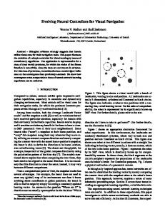
Figure 12: The dependence of heading estimation error rate on the number of features extracted. Dashed lines indicate that the given detector was unable to extract the number of keypoints required.

root-SIFT resulted in approximately 24% error, while the STAR-GRIEF error rate was around 2%. This indicates that the error rate improvement is caused by ability of the STAR-GRIEF to register images with large perceptual changes.

6.5. Number of features The error rate for estimating the correct heading is dependent on the number of extracted features, which depends on the setting of the ‘peak threshold’ of a particular feature detector. Our benchmarking software allows to select the detector peak thresholds in such a way that the detection method extracts a given number of features per image. To show the dependence of the heading estimation error on the number of features extracted, we evaluated the performance of the most popular image features set to extract {100, 200, . . . , 1600} features per dataset image. The results shown in Figure 12 demonstrate how the number of extracted features influences the ability of the method to correctly estimate the robot heading. Figure 12 also indicates that in some cases, it is not possible to reach a desired number of detected features (see the dashed lines). This is because the STAR detector does not extract enough features even if its peak threshold is set to the minimal value and the SpG detector was evaluated in three settings with 100, 220 and 740 features. The figure indicates that the lowest heading estimation error rates were achieved using the STAR/GRIEF and SpG/CNN image features. Figure 12 also shows that the performance of the features varies more for the North Campus and Stromovka datasets. This is caused by the fact that these datasets do not match images gathered on a monthly basis, but only from two opposite seasons, where the appearance changes are more prominent and the images are more difficult to register. To confirm this hypothesis, we divided the images of the Planetarium and Michigan datasets into two groups: ‘winter’ images, where the trees lack foliage and ‘summer’ images, where tree foliage is present. Then, we calculated the inter- and intra-season registration error rates of the upright-rootSIFT and STAR/GRIEF features. When matching images from the same season, both upright-root-SIFT and STAR-GRIEF methods achieved error rates below 3%. However, matching images across seasons by upright-

6.6. Combining different detectors and descriptors The performance of the image features is influenced by both the detector and descriptor phases. Although in some cases, the detection and description algorithms share the same data structures, which allows to speed up the feature’s calculation (such as the integral image in SURF), there is no reason why the detection and description phases of different algorithms could not be combined in order to obtain features with desired properties. For example, Matusiak and Skulimowski [57] report that the combination of the FAST detector and SIFT descriptor results in a computationally more efficient feature with similar robustness to the original SIFT. This lead us to test other detector/descriptor combinations of the features that we use. Tables 1 to 5 contain the error rates of the feature extractor algorithms obtained by combining different detectors and descriptors. The results summarized in Tables 1 to 5 confirm the high robustness of the STAR/GRIEF and SpG/CNN combinations to seasonal changes. Moreover, the results also indicate that the default detector/descriptor combinations are often not the best ones and one should consider alternative combinations. For example, exchanging the detector phase of the root-SIFT algorithm with the BRISK method dramatically improves invariance to seasonal changes. Due to the high computational costs of the CNN descriptor, we evaluated it only with the STAR and SpG detectors, since the first showed the best results with the other descriptors and the latter is a region detector particularly developed for combination with rich descriptors like CNN-based ones. 13

Table 1: Error rates of various detector/descriptor combinations in the Planetarium dataset, assuming 1600 features per image

Table 3: Error rates of various detector/descriptor combinations in the Stromovka dataset, assuming 1600 features per image

GRIEF rSIFT SURF FREAK CNN BRIEF SIFT BRISK ORB SpG1 STAR BRISK uSIFT SIFT uSURF SURF ORB FAST MSER GFTT

3.3 5.2 5.2 4.2 0.6 3.0 1.2 0.9 0.3 2.4 0.9 0.9 2.4 9.1 7.9 9.7 2.4 9.1 20.0 25.2 0.3 2.4 3.0 2.1 0.3 2.4 3.0 2.4 2.1 9.1 6.1 6.1 2.4 4.2 2.1 2.1 3.9 11.5 10.0 6.4 2.7 5.8 9.1 11.2

14.2 37.6 34.5 47.0 47.0 16.4 16.4 13.3 43.6 30.6 52.1

5.8 9.1 8.5 18.2 31.5 0.9 14.5 6.1 11.2 10.3 12.1

14.8 34.8 26.4 36.7 36.7 17.3 17.3 29.4 31.2 34.5 30.0

10.3 7.6 7.3 10.0 18.5 5.2 20.3 9.7 7.6 18.2 11.5

GRIEF rSIFT SURF FREAK CNN BRIEF SIFT BRISK ORB SpG1 16.4 STAR 5.0 BRISK 8.6 uSIFT 16.2 SIFT 16.2 uSURF 9.2 SURF 9.0 ORB 21.4 FAST 9.6 MSER 23.4 GFTT 10.4

0.0 2.1 — — — — — — — — —

6.7. Computational efficiency

26.0 13.0 15.0 23.4 23.4 12.8 12.8 28.8 12.8 39.6 19.6

9.8 11.2 7.2 24.0 40.8 8.0 15.2 11.8 17.2 26.6 25.0

10.2 9.4 7.0 25.8 45.4 7.8 13.6 12.2 14.0 21.8 24.6

36.0 64.2 60.2 68.4 68.4 42.8 42.8 27.6 63.2 63.8 65.8

18.4 34.6 25.8 44.2 58.8 12.8 42.2 20.6 30.8 35.6 36.6

28.8 60.2 45.8 65.4 65.4 36.2 36.2 43.8 54.4 59.2 59.4

34.0 30.0 32.6 30.2 45.4 29.8 57.8 23.2 26.2 51.6 27.2

5.2 8.6 — — — — — — — — —

An important property of an image feature is the amount of processing time required for its extraction from an image and the amount of time it takes to match it to the map. In our evaluations, we calculated the times it takes to detect, describe and match the given features and normalized this time per 1000 features extracted. The estimate is only coarse because the time required for feature detection is more dependent on the image size than on the number of features and the feature matching speed can be boosted by techniques like approximate nearest neighbour [58]. Moreover, detec-

tors and descriptors of the same features often share data structures, which means that if used together, the time for their extraction is lower then the sum of the detection and description times indicated in Table 6. However, the statistics shown in Table 6 are still useful to rank the algorithms according to their computational efficiency. The Table 6 shows the times to extract and match the conventional image features on an i7 processor and the CNN features on an NVidia Titan X GPU. We omitted the upright variants of SIFT and SURF as well as root SIFT, because their computational time is the same. The computational complexity of the GRIEF

Table 2: Error rates of various detector/descriptor combinations in the Michigan dataset, assuming 1600 features per image

Table 4: Error rates of various detector/descriptor combinations in North Campus dataset, assuming 1600 features per image

GRIEF rSIFT SURF FREAK CNN BRIEF SIFT BRISK ORB SpG1 1.5 4.5 6.1 7.9 STAR 1.8 4.5 6.1 6.7 BRISK 1.5 3.0 3.9 5.5 uSIFT 8.5 9.7 9.4 10.6 SIFT 8.5 9.7 13.0 15.8 uSURF 1.5 2.4 7.3 8.5 SURF 1.5 2.4 3.9 5.5 ORB 15.5 20.0 24.8 28.5 FAST 7.3 8.8 8.5 9.1 MSER 16.1 21.8 13.6 15.5 GFTT 9.4 9.1 7.6 10.3 1 The

9.4 23.9 14.2 35.2 35.2 8.8 8.8 25.8 20.9 27.6 36.4

1.5 9.1 3.0 13.0 16.7 2.1 5.8 18.8 6.1 14.5 9.7

3.3 13.9 12.1 27.9 27.9 3.3 3.3 24.2 15.2 32.4 22.1

7.9 3.9 4.2 11.5 7.6 5.8 8.2 20.9 9.4 21.8 14.2

GRIEF rSIFT SURF FREAK CNN BRIEF SIFT BRISK ORB SpG1 9.5 STAR 5.8 BRISK 6.1 uSIFT 16.7 SIFT 16.7 uSURF 6.3 SURF 6.1 ORB 25.8 FAST 15.6 MSER 27.3 GFTT 19.7

0.3 1.8 — — — — — — — — —

1 The

Superpixel Grid detector (SpG) used 740 keypoints.

14

11.7 10.2 8.0 25.2 25.2 7.6 7.6 34.9 18.7 36.2 25.8

9.1 8.0 6.1 27.1 40.3 8.2 11.9 31.2 20.2 23.0 28.9

10.6 8.9 6.7 30.4 42.5 9.5 13.2 31.9 21.9 24.3 31.7

19.9 37.3 28.4 54.4 54.4 21.2 21.2 45.6 51.6 46.2 63.3

9.1 13.2 10.8 29.1 39.0 6.1 20.6 27.6 26.0 26.0 32.5

21.7 37.7 32.8 48.4 48.4 17.1 17.1 53.4 47.5 48.4 53.8

Superpixel Grid detector (SpG) used 740 keypoints.

17.8 14.7 13.2 27.8 36.4 8.3 17.4 31.2 25.0 37.3 32.1

4.1 4.3 — — — — — — — — —

Table 5: Error rates of various detector/descriptor combinations in Nordland dataset, assuming 1600 features per image

over, matching 1000 CNN descriptors takes more than a second, which is also significantly slower compared to the classic features. However, matching could be speeded up by techniques tailored for high-dimensional descriptors, e.g. binary locality-sensitive hashing [59].

GRIEF rSIFT SURF FREAK CNN BRIEF SIFT BRISK ORB SpG1 5.1 6.7 1.3 1.5 6.7 5.5 8.6 21.9 STAR 0.4 1.7 1.7 1.3 18.7 2.5 9.0 7.8 BRISK 0.6 0.6 0.8 1.0 13.9 1.0 1.9 4.6 uSIFT 1.3 0.6 1.3 1.0 28.8 2.9 4.4 2.9 SIFT 1.3 0.6 2.9 2.9 28.8 6.9 4.4 2.5 uSURF 0.4 1.0 1.1 0.8 2.9 0.4 1.9 5.0 SURF 0.4 1.0 2.1 1.7 2.9 2.3 1.9 8.0 ORB 5.7 4.0 4.4 4.2 3.4 4.0 11.6 5.9 FAST 0.6 0.6 1.1 1.1 11.6 1.1 2.5 2.1 MSER 45.9 50.3 25.5 24.2 51.8 47.2 60.2 58.1 GFTT 2.1 2.1 1.7 2.3 33.5 2.7 3.2 5.0 1 The

0.9 1.3 — — — — — — — — —

6.8. Discussion The results presented in Sections 6.5 to 6.7 indicate that the CNN-based descriptors in combination with the Superpixel Grid detector achieve low error rates even with a low number of detected features. When using a large number of keypoints, the performance of the SpG/CNN and STAR/GRIEF features evens out, and they both achieve low heading estimation error rates. While the SpG/CNN performs better on the Michigan, North Campus and Planetarium datasets, which contain a higher number of man-made structures, the STAR/GRIEF achieves lower errors on the Stromovka and Nordland datasets, which contain a larger amount of foliage that exhibits significant appearance changes due to seasonal factors. Compared to the CNN features, the GRIEF is much faster to calculate even on an ordinary CPU. Our analysis assumes a teach-and-repeat scenario, where a robot moves along a previously-taught path and thus, the visual navigation method does not have to be robust to large viewpoint changes. In a realistic scenario, a robot might have to deviate from the taught path, e.g. due to an obstacle. In order to deal with these situations, the image features used should still be able to handle small-scale viewpoint changes. Experiments with ground [56] and aerial [60] robots have shown that teach-and-repeat systems based on the STAR/BRIEF feature routinely deal with position deviations of up to 1 meter. Unlike SpG/CNN, which is designed for general use, the STAR/GRIEF combination is not meant to handle large viewpoint changes and one should be cautious when applying it for general long-term navigation and localisation. For example, [61] evaluated the performance of several image features in a scenario of lakeshore monitoring, where the on-board camera aims perpendicularly to the vehicle movement and thus, the viewpoint changes are significant. The authors of [61] concluded that in their scenario, the ORB feature, which is based on BRIEF, slightly outperformed the other features.

Superpixel Grid detector (SpG) used 740 keypoints.

Table 6: Time required to detect, describe and match 1000 features by the feature extractors used in our evaluation

Method SIFT SURF BRISK ORB BRIEF GRIEF FREAK CNN-CPU CNN-GPU MSER GFTT STAR FAST SPGrid

Time [ms] required to detect describe match 200 99 63 8 – – – – – 75 16 16 9 49

64 63 5 6 3 3 15 33000 3100 – – – – –

85 93 64 58 63 60 58 1650 1650 – – – – –

descriptor is the same as the BRIEF one, which is not surprising because these two algorithms differ only in the choice of pixel positions used for brightness comparisons. Table 6 shows that the combination of the STAR detector and (G)BRIEF descriptor is computationally inexpensive not only for the extraction itself, but also for matching. It also indicates that the CNN descriptor is computationally expensive – calculation of a single descriptor takes 3ms on a GPU, which is three orders of magnitude longer than BRIEF. More-

7. Conclusion We report our results on the evaluation of image feature extractors to mid- and long-term environment 15

References

changes caused by variable illumination and seasonal factors. Our evaluation was taken from the navigational point of view – it was based on the feature extractors’ ability to correctly establish the robot’s orientation, and hence, keep it on the intended trajectory. The datasets used for evaluation capture seasonal appearance changes of three outdoor environments from two different continents. Motivated by previous works which indicated that certain combinations of feature detectors and descriptors outperform commonly used features, we based our evaluation on combinations of publicly-available detectors and descriptors. For example, substituting the detection phase of the root-SIFT algorithm with the BRISK method dramatically improves its invariance to seasonal changes, while making the algorithm computationally more efficient. We noted that the BRIEF descriptor based on bitwise comparisons of the pixel intensities around a keypoint detected by the STAR method performed better than most other detector/descriptor combinations. To further elaborate on this result, we trained the comparison sequences that constitute the core of the BRIEF descriptor on a limited number of images, obtaining a new feature, which we call GRIEF. The lowest registration error rates (2.4% and 3.0%) were achieved by the SpG/CNN and STAR/GRIEF detector/descriptor combinations, which makes these features a good choice for vision-based teach-and-repeat systems operating in outdoor environments for long periods of time. While the SpG/CNN performed better in semi-urban areas, the performance of STAR/GRIEF was slightly higher in environments with natural features such as foliage, where it was trained on. Moreover, the STAR/GRIEF feature was faster to calculate, which makes it suitable even for resource-constrained systems. We hope that this evaluation will be useful for other researchers concerned with long-term autonomy of mobile robots in challenging environments and will help them to choose the most appropriate image feature extractor for their navigation and localization systems. To allow further analysis of this problem, we provide the aforementioned benchmarking framework and the GRIEF training method as a documented, open-source software package [21].

[1] J. Li, N. Allinson, A comprehensive review of current local features for computer vision, Neurocomputing. [2] K. Mikolajczyk, C. Schmid, A performance evaluation of local descriptors, IEEE Transactions on Pattern Analysis and Machine Intelligence 27 (10) (2005) 1615–1630. doi:10.1109/TPAMI.2005.188. [3] D. Mukherjee, Q. JonathanWu, G. Wang, A comparative experimental study of image feature detectors and descriptors, Machine Vision and Applications (2015) 1–24doi:10.1007/s00138015-0679-9. [4] D. G. Lowe, Distinctive image features from scale-invariant keypoints, Int. J. Comput. Vision 60 (2) (2004) 91–110. [5] S. Gauglitz, T. H¨ollerer, M. Turk, Evaluation of interest point detectors and feature descriptors for visual tracking, International journal of computer vision 94 (3) (2011) 335–360. [6] A. Gil, O. Mozos, M. Ballesta, O. Reinoso, A comparative evaluation of interest point detectors and local descriptors for visual SLAM, Machine Vision and Applications (2010) 905– 920doi:10.1007/s00138-009-0195-x. [7] S. Lowry, N. Sunderhauf, P. Newman, J. Leonard, D. Cox, P. Corke, M. Milford, Visual place recognition: A survey, IEEE Transactions on Robotics, PP (99) (2015) 1–19. doi:10.1109/TRO.2015.2496823. [8] N. Sunderhauf, S. Shirazi, A. Jacobson, F. Dayoub, E. Pepperell, B. Upcroft, M. Milford, Place recognition with convnet landmarks: Viewpoint-robust, condition-robust, training-free, Robotics: Science and Systems XII. [9] W. Churchill, P. Newman, Practice makes perfect? managing and leveraging visual experiences for lifelong navigation, in: ICRA, 2012. [10] P. Furgale, T. D. Barfoot, Visual teach and repeat for long-range rover autonomy, Journal of Field Robotics. [11] T. Krajn´ık, J. Faigl, V. Von´asek et al., Simple, yet Stable Bearing-only Navigation, Journal of Field Robotics. [12] Z. Chen, S. T. Birchfield, Qualitative vision-based path following, IEEE Transactions on Robotics and Automationdoi:http://dx.doi.org/10.1109/TRO.2009.2017140. [13] C. Valgren, A. J. Lilienthal, SIFT, SURF & seasons: Appearance-based long-term localization in outdoor environments, Robotics and Autonomous Systems 58 (2) (2010) 157– 165. [14] E. Royer, M. Lhuillier, M. Dhome, J.-M. Lavest, Monocular vision for mobile robot localization and autonomous navigation, Int. Journal of Computer Vision. [15] M. Calonder, V. Lepetit, C. Strecha, P. Fua, BRIEF: binary robust independent elementary features, in: ICCV, 2010. [16] E. Rublee, V. Rabaud, K. Konolige, G. Bradski, ORB: An Efficient Alternative to SIFT or SURF, in: International Conference on Computer Vision, Barcelona, 2011. [17] S. Leutenegger, M. Chli, R. Y. Siegwart, Brisk: Binary robust invariant scalable keypoints, in: 2011 International conference on computer vision, IEEE, 2011, pp. 2548–2555. [18] P. Neubert, P. Protzel, Local region detector+ CNN based landmarks for practical place recognition in changing environments, in: ECMR, IEEE, 2015, pp. 1–6. [19] T. Krajn´ık, P. Crist´oforis, M. Nitsche, K. Kusumam, T. Duckett, Image features and seasons revisited, in: European Conference on Mobile Robots (ECMR), IEEE, 2015, pp. 1–7. [20] N. Carlevaris-Bianco, A. K. Ushani, R. M. Eustice, University of Michigan North Campus long-term vision and lidar dataset, The International Journal of Robotics Research. [21] T. Krajn´ık, GRIEF source codes and benchmarks. URL http://purl.org/robotics/grief-code

Acknowledgments The work has been supported by the EU ICT project 600623 ‘STRANDS’ and UBACYT project 20020130300035BA. We would like to thank Nicholas Carlevaris-Bianco for sharing the Michigan dataset. 16

[22] G. D. Finlayson, S. D. Hordley, Color constancy at a pixel, Journal of the Optical Society of America: Optics, image science, and vision 18 (2) (2001) 253–64. [23] W. Maddern, A. D. Stewart, C. McManus, B. Upcroft, W. Churchill, P. Newman, Illumination invariant imaging: Applications in robust vision-based localisation, mapping and classification for autonomous vehicles, in: ICRA Workshop on Visual Place Recognition in Changing Environments, 2014. [24] C. McManus, W. Churchill, W. Maddern, A. Stewart, P. Newman, Shady dealings: Robust, long-term visual localisation using illumination invariance, in: International Conference on Robotics and Automation (ICRA), 2014, pp. 901–906. [25] K. MacTavish, M. Paton, T. Barfoot, Beyond a shadow of a doubt: Place recognition with colour-constant images, in: Field and Service Robotics (FSR), 2015. [26] M. Paton, K. MacTavish, C. Ostafew, T. Barfoot, It’s not easy seeing green: Lighting-resistant stereo visual teach-and-repeat using color-constant images, in: International Conference on Robotics and Automation (ICRA), 2015. [27] J. Mount, M. Milford, 2d visual place recognition for domestic service robots at night, in: International Conference on Robotics and Automation (ICRA), 2016. [28] F. Dayoub, T. Duckett, An adaptive appearance-based map for long-term topological localization of mobile robots, in: IROS, 2008. [29] D. M. Rosen, J. Mason, J. J. Leonard, Towards lifelong featurebased mapping in semi-static environments, in: International Conference on Robotics and Automation (ICRA), IEEE, 2016. [30] N. Carlevaris-Bianco, R. M. Eustice, Learning visual feature descriptors for dynamic lighting conditions, in: IEEE/RSJ Int. Conference on Intelligent Robots and Systems (IROS), 2014. [31] S. Lowry, G. Wyeth, M. Milford, Unsupervised online learning of condition-invariant images for place recognition, Australasian Conference on Robotics and Automation 2014. [32] T. Cieslewski, E. Stumm, A. Gawel, M. Bosse, S. Lynen, R. Siegwart, Point cloud descriptors for place recognition using sparse visual information. [33] S. Lowry, M. Milford, G. Wyeth, Transforming morning to afternoon using linear regression techniques, in: International Conference on Robotics and Automation (ICRA),, IEEE, 2014. [34] P. Neubert, N. S¨underhauf, P. Protzel, Appearance change prediction for long-term navigation across seasons, in: ECMR, 2013. [35] N. S¨underhauf, P. Neubert, P. Protzel, Predicting the change– a step towards life-long operation in everyday environments, Robotics Challenges and Vision (RCV2013). [36] T. Krajnik, J. Fentanes, G. Cielniak, C. Dondrup, T. Duckett, Spectral analysis for long-term robotic mapping, in: International Conference on Robotics and Automation (ICRA), 2014. [37] T. Krajn´ık, J. P. Fentanes, O. M. Mozos, T. Duckett, J. Ekekrantz, M. Hanheide, Long-term topological localization for service robots in dynamic environments using spectral maps, in: Int. Conf. on Intelligent Robots and Systems (IROS), 2014. [38] C. McManus, B. Upcroft, P. Newmann, Scene signatures: localised and point-less features for localisation, in: RSS, 2014. [39] T. Krajn´ık, S. Pedre, L. Pˇreuˇcil, Monocular Navigation System for Long-Term Autonomy, in: International Conference on Advanced Robotics (ICAR), 2013. [40] N. S¨underhauf, F. Dayoub, S. Shirazi, B. Upcroft, M. Milford, On the performance of convnet features for place recognition, arXiv preprint arXiv:1501.04158. [41] N. Sunderhauf, P. Corke, Visual place recognition in changing environments (VPRiCE), https://roboticvision. atlassian.net/wiki/pages/viewpage.action? pageId=14188617.

[42] D. Mishkin, M. Perdoch, J. Matas, Place recognition with WxBS retrieval, in: CVPR 2015 Workshop on Visual Place Recognition in Changing Environments, 2015. [43] K. Mikolajczyk, C. Schmid, An affine invariant interest point detector, in: European Conference on Computer Vision, 2002. [44] J. Matas, O. Chum, M. Urban, T. Pajdla, Robust wide-baseline stereo from maximally stable extremal regions, Image and vision computing 22 (10) (2004) 761–767. [45] E. Rosten, T. Drummond, Machine learning for high-speed corner detection, in: European Conf. on Computer Vision, 2006. [46] E. Mair, G. D. Hager, D. Burschka, M. Suppa, G. Hirzinger, Adaptive and generic corner detection based on the accelerated segment test, in: European Conference on Computer Vision, 2010. [47] M. Agrawal, K. Konolige, M. R. Blas, Censure: Center surround extremas for realtime feature detection and matching, in: European Conf. on Computer Vision (ECCV), Springer, 2008, pp. 102–115. [48] P. Neubert, P. Protzel, Beyond holistic descriptors, keypoints, and fixed patches: Multiscale superpixel grids for place recognition in changing environments, IEEE Robotics and Automation Letters 1 (1) (2016) 484–491. doi:10.1109/LRA.2016.2517824. [49] R. Arandjelovi´c, A. Zisserman, Three things everyone should know to improve object retrieval, in: Computer Vision and Pattern Recognition (CVPR), 2012, pp. 2911–2918. [50] H. Bay, A. Ess, T. Tuytelaars, L. Van Gool, Speeded-up robust features (SURF), Computer Vision and Image Understanding. [51] A. Alahi, R. Ortiz, P. Vandergheynst, Freak: Fast retina keypoint, in: IEEE conference on Computer vision and pattern recognition (CVPR), IEEE, 2012. [52] K. Chatfield, K. Simonyan, A. Vedaldi, A. Zisserman, Return of the devil in the details: Delving deep into convolutional nets, in: British Machine Vision Conference, 2014. [53] M. A. Fischler, R. C. Bolles, Random sample consensus: A paradigm for model fitting with applications to image analysis and automated cartography, Commun. ACM (1981) 381– 395doi:10.1145/358669.358692. [54] Stromovka dataset, [Cit: 2013-03-25]. URL http://purl.org/robotics/stromovka_dataset [55] D. G. R. Bradski, A. Kaehler, Learning Opencv, 1st Edition, 1st Edition, O’Reilly Media, Inc., 2008. [56] P. De Crist´oforis, M. Nitsche, T. Krajn´ık, T. Pire, M. Mejail, Hybrid vision-based navigation for mobile robots in mixed indoor/outdoor environments, Pattern Recognition Letters. [57] K. Matusiak, P. Skulimowski, Comparison of key point detectors in sift implementation for mobile devices, Computer Vision and Graphics (2012) 509–516. [58] E. Kushilevitz, R. Ostrovsky, Y. Rabani, Efficient search for approximate nearest neighbor in high dimensional spaces, SIAM Journal on Computing 30 (2) (2000) 457–474. [59] M. S. Charikar, Similarity estimation techniques from rounding algorithms, in: Proceedings of the thiry-fourth annual ACM symposium on Theory of computing, ACM, 2002, pp. 380–388. [60] M. Nitsche, T. Pire, T. Krajn´ık, M. Kulich, M. Mejail, Monte carlo localization for teach-and-repeat feature-based navigation, in: Towards Autonomous Robotics Systems (TAROS), 2014. [61] S. Griffith, C. Pradalier, Survey registration for long-term natural environment monitoring, Journal of Field Robotics.

17