Planar Image Based Visual Servoing as a Navigation ... - CiteSeerX

Planar Image Based Visual Servoing as a Navigation Problem∗ Noah J. Cowan and Daniel E. Koditschek Electrical Engineering and Computer Science The University of Michigan Ann Arbor, MI 48105-2110 E-mail: {ncowan, kod}@eecs.umich.edu

Abstract

is generally only guaranteed locally [18, 19] (with the exception of a few algorithms for point positioning and estimation problems [9, 17]). Conversely, one easily specifies an essentially globally convergent controller using task space error coordinates, but when using PB servoing the controller must also avoid occlusions or risk losing site of the features necessary for pose estimation.

We describe a hybrid planar image-based servo algorithm which, for a simplified planar convex rigid body, converges to a static goal for all initial conditions within the workspace of the camera. This is achieved using the sequential composition of a palette of continuous image based controllers. Each subcontroller, based on a specified set of collinear feature points, is shown to converge for all initial configuations in which the feature points are visible. Furthermore, the controller guarantees that the body will maintain a “visible” orientation, i.e. the feature points will always be in view of the camera. This is achieved by introducing a change of coordinates fromPSfrag SE(2) replacements to an image plane measurement of three points, and imposing a navigation function in that coordinate system. Our intuition suggests that appropriately generalized versions of these ideas may be extended to SE(3).

yb π2 π1 −ζE

1

Introduction

Visual servoing describes a broad class of problems in which a robot is positioned with respect to a target using computer vision as the primary feedback sensor [4, 6, 7, 9, 14]. There are traditionally two approaches to visual servoing: 2D image-based (IB), and 3D position based (PB). In image-based visual servoing the control objective is to minimize the perceived error (i.e. image plane error), whereas the objective in position-based visual servoing is to minimize the task space error. It is accepted that IB is more robust with respect to calibration uncertainty than PB servoing, though to our knowledge this has never been formally justified. The disadvantage of IB servoing is that convergence ∗ This work was supported in part by the NSF under grant IRI-9510673

xb π3

z1 z2

z3 +ζE

yc α

xc

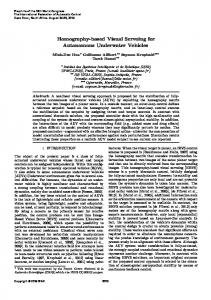
Figure 1: The objective is to drive the rigid body so that each feature aligns with the respective feature on a goal image, while avoiding collisions with ±ζE . The first portion of the algorithm requires three features (depicted by +, × and •) visible on the body and on the goal, a condition not always satisfied. The “simple-minded” workaround is to “hallucinate” the occluded feature for the controller. We prefer to work only with the visible features available at each position, as depicted in Figure 2.

1.1

Motivation

The long term aim of our research seeks to develop a system that couples visual estimation of a dynamical rigid body with visual servoing of a robot manipulator in order to achieve a dynamical task, such as catching an otherwise unsensed falling body, or snatching an object from a conveyor. Our approach to such problems presupposes well designed robust “early vision” algorithms [5, 8] that track features such as corners and edges of the objects being observed. This affords the use of a growing body of signal processing algorithms designed to identify such features of an image and models the camera as a virtual sensor providing image plane coordinates for the objects being observed. Hutchinson et. al. provide a tutorial introduction to this approach [7]. As a rigid body moves in space, actuated or not, its corners and edges typically cycle into and out of the view of the cameras. Consequently it will often be necessary to switch the focus of attention during motion, introducing a hybrid aspect to the problem. The natural place to detect occlusions is the image plane, which argues for using the IB approach. To achieve stable and robust systems, therefore, it is desirable to develop IB algorithms with large domains of attraction in order to simplify the challenging and inevitable hybrid switching problem that results. The present effort tackles a simplified version of image-based servoing in which the “world” is a plane, and the camera is one dimensional. The rigid body under control thus possesses three degrees of freedom and may be represented as a point in SE(2). However, our interest lies not merely in the application to planar problems, but in the generalization of these techniques to six-degree-of-freedom bodies moving in SE(3) with two dimensional cameras. Our intuition suggests that there should be an appropriate generalization of this body of theory to that case.

1.2

Relation to Existing Literature

Much of the recent literature [6, 18, 19] uses local linearizations to solve tracking and servoing problems for both points and 3D objects. Some recent papers from our laboratory [9, 17] present algorithms, stability analysis and a working implementation [9] of systems with provably large domains of attraction for point positioning and estimation – i.e. necessarily without recourse to local linearizations. One group has recently presented a convergent rigid body visual servoing algorithm, dubbed “2D 1/2” visual servoing since it is between IB (2D) and PB (3D) [14]. This

clever idea uses the homography between sets of corresponding points in the current image and the desired image at each iteration to compute an approximate partial pose error from which the control law is derived.

1.3

Contributions

This paper aims to overcome the local limitations of IB servos by addressing a simplified planar visual servo problem. In particular, we assume that three collinear edge features of a fully actuated planar rigid body are viewed by a one dimensional camera (see Figure 1). With the simple observation that there is a diffeomorphism between an appropriate subset of the space of rigid transformations, SE(2), and the space of “visible” triples of image plane measurements, I, the problem of image plane servoing in this setting reduces to the problem of stringing beads on a wire: move the three image plane points to their respective goals while avoiding collisions with each other and with the edge of the image plane. A navigation function1 [16] was first introduced by the second author [12] which solves the latter problem. By an appropriate extension of that navigation function in the present context, convergence to the goal is guaranteed for all initial conditions in which the three feature points are visible. Using a sequential composition technique proposed in [2], this is extended to include all initial conditions in the camera’s workspace.

2

Planar Rigid Body Servos

Our stated objective is to design an IB visual servo system for control of a planar convex polygonal rigid body which directly minimizes the “percieved error,” such that all initial conditions in the camera workspace converge to the goal. Such a controller must, by its very nature, be hybrid since not all faces of the body are visible in all configurations within the camera workspace. We address the hybrid problem in two steps: 1. Design an IB visual servo controller, Φ, to have as its domain of attraction those initial conditions in which the same features are visible (a notion to be 1 Strictly speaking, a navigation function [15] is an artificial potential function on a compact set which has no spurious minima, evaluates to 1 on the boundary and evaluates uniquely to zero at the goal. Clearly SE(2) is not compact, but using a diffeomorphism motivated by the camera projection we first compactify a subset of SE(2) to a subset of the compact torus T3 .

formally defined later) on the body as on the goal image. Furthermore, make such configurations positive invarient, so that once in view, the body must reach the goal while still visible. 2. Design a palette of controllers with appropriately overlapping domains of attraction and an IB switching law which renders the entire camera workspace as the composite domain of attraction for the final goal state. Section 2.1 formally defines the problem and introduces some notation. In Section 2.2 we address Step 1 above by establishing a formal change of coordinates from task space coordinates to image plane coordinates, and pose a navigation function on the image plane which is pulled back to the task for implementation. Facilitated by the large parameterized and exactly bounded domain of attraction achieved using navigation functions, Section 2.3 outlines our approach to solving Step 2 by recourse to sequential backchaining. It may be useful to review the notation in Appendix A before proceeding.

2.1 2.1.1

2.1.2

Camera Model

The pinhole camera model (Figure 1) has lent theoretical and practical utility to previous work in our laboratory [9, 17] and we exploit its simple structure in the present effort. Define a fixed world coordinate system with two axes denoted {xc , yc } such that the yc -axis is orthogonal to the image plane,3 and the origin is at the camera pinhole. The camera is assumed to have an aperture, α ∈ (−π/2, π/2), which defines the workspace of the camera  Wc = d ∈ A2 : d2 > 0, arctan (d1 /d2 ) ∈ (−α, α) .

The planar pinhole camera map γ : Wc → R is simply d1 (4) γ(d) = λ . d2

where λ ∈ R+ is the camera focal length and d is expressed in camera coordinates. The “edge” of the image plane corresponds to the two points ±ζE where ζE = λ tan α

(5)

i.e.

Problem Setup

γ(Wc ) = (−ζE , ζE ).

Plant Model

The configuration of a planar rigid body may be written in terms of a homogeneous transformation matrix H ∈ SE(2). We will adopt the convention that if p ∈ A2 is a point in a body-fixed coordinate system, then Hp is the same point with respect to a global coordinate system. For simplicity,2 we posit a purely kinematic plant model, i.e. we assume the robotic systems moving the ridig body accepts velocity control. Now choose a set of local coordinates   qθ ∈ R3 (1) q= qr such that H = ψ(q) = H0



exp {Jqθ } 0T

qr 1



, J=



0 1

−1 0

 (2)

where H0 ∈ SE(2) is fixed. The plant model in these coordinates is q˙ = u (3) The control objective is to drive q → q ∗ as t → ∞. 2 Recourse

to a kinematic plant model is purely for clarity of presentation in the present work – by using navigation functions we will automatically inherit a second order dynamic controller as well [10, 11].

2.1.3

Rigid Bodies and “Visibility”

Consider a planar convex polygonal rigid body H ∈ SE(2) whose goal state is H ∗ = ψ(q ∗ ) ∈ SE(2), i.e. the control objective is to drive H → H ∗ as t → ∞. Let pi ∈ A2 , i = 1, 2, 3, denote three distinct points on the same edge,4 E, with respect to a body fixed coordinate system. We choose the body coordinate system axes {xb , yb } such that the “xb -axis” is coincident with the edge on which the three points lie and the “yb -axis” points “toward” the body as depicted in Figure 2. Hence, the three points can be expressed as   p1 , p2 , p3 ∈ (A2 )3 , P = p~i = πi e1 , where the πi ’s are distinct. We also assert with no loss of generality that πi < πj for i < j. Note that Hpi expresses the ith point in camera (world) coordinates. Of course not all positions and orientations of the rigid body allow a clear view of the feature points by the camera. Hence it will facilitate the discussion to 3 Since the “world” is chosen to be a plane, the camera image is one dimensional, so the image plane is really a line. 4 We presume that this machinery will work for 3 noncollinear points as well, though our analysis for the case in which they are collinear is complete and hence it is presented here.

H ∈F H∈ /W =⇒ H ∈ /V

H∈ /F H ∈W =⇒ H ∈ /V

H ∈F H ∈W =⇒ H ∈ V

xb yb

replacements

xb yb

yb

xb

z1

z3 z2 z1

z2 z3

z1 z2

z3

Figure 2: A cartoon depiction of the sets F, W and V. For simplicity, the image plane is drawn in front of the camera pinhole. From left to right, the figures show three typical configurations of a rigid body with respect to a planar camera. Left: The edge is facing the camera, but the leftmost point is out of view. Center: Although completely within the camera workspace, the edge is facing away from the camera and is occluded by the body. Right: The edge is facing and within the field of view of the camera. introduce two sets. Informally, let F denote the set of orientations in SE(2) such that E is “facing” the camera. Likewise, denote by W the set of orientations that keeps the feature points within the aperture (or workspace) of the camera. These sets are illustrated in Figure 2. To define F formally it will be useful to develop a physical notion of “facing the camera” in terms of a function v : SE(2) → R v(H) := −rT J T Re1 where H=



R 0T

r 1



(6)

.

Note that J T Re1 is the edge normal vector pointing out of the body and that v(H) = 0 if and only if the points represented by HP are collinear with the camera origin, o = [0, 0, 1]T , that is to say HP − [o, o, o] has rank 1 (B). Define the set of orientations “facing” the camera F ⊂ SE(2) F := {H ∈ SE(2) : v(H) > 0} .

(7)

An important fact is that if H ∈ F then Hpi 6= o, i = 1, 2, 3 (Appendix B). We may now define the workspace of the rigid body W = {H ∈ SE(2) : Hpi ∈ Wc , i = 1, 2, 3} .

Finally, we denote the “visible” set V =F ∩W and define our virtual sensor c : V → R3   γ(Hp1 ) c(H) =  γ(Hp2 )  γ(Hp3 )

(8)

(9)

where γ is given in (4). Denote the range of V under c as I := c(V) ⊂ R3 . Note that  I = z ∈ R3 : − ζE < z1 < z2 < z3 < ζE . (10)

2.2

Image Plane Navigation

Recall that our objective is to design a feedback system which minimizes the percieved error i.e. we desire to drive z → z ∗ as t → ∞, where z = c(H) and z ∗ = c(H ∗ ). Our approach to image-based servoing is motivated by the following observation: it is possible to force our features to navigate the image plane coordinates, and “pull that result back” to the physical task space, SE(2), without ever requiring a direct reconstruction of that physical situation.5 5 Of

course, as is usually the case in image-based visual ser-

2.2.1

2.2.2

Navigation Function

We have shown that c is a diffeomorphism between V and that its image I [3]. Since c is a diffeomorphism we may freely drive z, so long as we stay in I (c is not a valid diffeomorphism outside of I). In other words, we reduce the problem of planar IB servoing to the problem of using feedback to drive three points on a line to their respective goals, while avoiding collisions between each other or with the “edge” of the image plane. Define the following “blow-up”6 b : I → R3   β(z1 ) b(z) =  β(z2 )  (11) β(z3 ) where β : γ(Wc ) → R is a diffeomorphism whose range is all of R. Note that b is a diffeomorphism, and that its image is  B+ := b(I) = y ∈ R3 : y1 < y2 < y3 .

(12)

Assume that H ∗ ∈ V, and let y ∗ = b◦c(H ∗ ). Define the objective function ϕ e : B+ → [0, ∞) (parameterized by y ∗ ) (y1 − y1∗ )2 + (y2 − y2∗ )2 + (y3 − y3∗ )2 ϕ ey∗ (y) = (y1 − y2 )2 (y1 − y3 )2 (y2 − y3 )2


k

.

(13) Since this objective function blows up at the obstacles, we “squash” it with σ : [0, ∞) → [0, 1) σ(u) =

u1/k . (1 + u)1/k

(14)

According to the second author [12], ey∗ . ϕ¯y∗ = σ ◦ ϕ

(15)

is a navigation function on B+ for k > 7/2, which we now assume. But since b ◦ c is a diffeomorphism between V and B+ , we have that the pull back of ϕ¯ to V (16) , ϕy∗ = ϕ¯y∗ ◦ b ◦ c, is a navigation function on V [15]. voing, some information about the physical situation is needed to compute Dc, the Jacobian matrix of c. In practice, depth estimates may be computed by one of the many pose estimation algorithms, as found for example in [13]. 6 This choice is somewhat arbitrary and may be chosen freely up to the constraints listed. One might choose, for example β(ζ) = ζ/(ζE2 − ζ 2 ).

Image-Based Controller

Since ϕ is a navigation function on V, the controller  q˙ = u Φ := (17) u = −(Dq ϕy∗ ◦ ψ )T renders V as the domain of attraction for unique stable critical point H ∗ . The controller, Φ, depends on 1. The virtual sensor, c, which depends on choice of the edge, E, and its feature points. 2. The goal, H ∗ , through the image of the goal feature points y ∗ = c(H ∗ ). We will write Φ(E, H ∗ ) to make the dependances explicit. Finally, let D(Φ) denote the domain of attraction of Φ around the goal G(Φ). For this controller, D(Φ) = V and G(Φ) = H ∗ .

2.3

Sequential Composition

In this section, we use sequential composition to construct a hybrid “global” image-based servo for a planar rigid body. A detailed and general procedure for applying sequential composition is outlined in [2], so we conclude for the sake of clarity with a simple example in which the rigid body is a triangle. The idea can easily be extended to a convex polygonal body with n edges. 2.3.1

Example: Triangular Body

Consider a triangle with edges labeled E0 , E1 , E2 , each of which has three distinguishable feature points. We now seek a “global” hybrid controller to drive the body to a specified goal for all initial conditions for which at least one edge of the rigid body starts out in view of the camera. For each edge, define Vi to be the set in which the ith edge is visible in the manner described in Section 2.1.3. Also, each edge gives rise to a different virtual sensor, ci : Vi → R3 , namely the projection of the features on the ith edge to the image plane. Just as we have assumed that individual features are mutually distinguishable, we will assume that each set of edge features is also mutually distinguishable. Let H0∗ denote the final goal and assume that H0∗ ∈ V0 . Place two subgoals, H1∗ and H2∗ such that H1∗ ∈ V0 ∩ V1 , H2∗ ∈ V1 ∩ V2 .

(18)

For example, one may place H1∗ such that the vertex between E0 and E1 lies along the positive yc -axis far

enough from the camera that the body is fully within the camera workspace and oriented so that both edges are in view (likewise with H2∗ ). Now, define three image-based controllers Φ0

:= Φ(E0 , H0∗ )

Φ1 Φ2

:= Φ(E1 , H1∗ ) := Φ(E2 , H2∗ ).

Note that the domains of attraction and goals of these controllers are shown in Table 1.

Φ0 Φ1 Φ2

D V0 V1 V2

G H0∗ H1∗ H2∗

Table 1: This shows the domain of attraction and goal for each of the three controllers, Φ0 , Φ1 and Φ2 . Following Burridge et. al. [1, 2] we say that controller Φi prepares controller Φj , written Φi  Φj , if G(Φi ) ∈ D(Φj ). In our case, we have Φ2  Φ 1  Φ 0 .

(19)

Given this palette of image-based controllers it is now possible to design a single hybrid switching controller, by simply assigning priority to the individual controllers. Priority assignment in this case is trivial; we simply assign Φ0 to have the highest priority, Φ1 the second highest and Φ2 the lowest. This ordering induces a directed acyclic graph. The result of such a switching controller is to drive all initial conditions in which at least one of the three edges is in view to the goal, and hence we have a “global” image-based controller.

3

Conclusion

We have presented a hybrid controller for rigid body servoing which uses sequential composition to compose a palette of image-based visual servo controllers. The central contribution of this paper lies in the construction of a parametrized set of image-based controllers based on navigation functions. The large and exactly bounded domain of attraction of each controller facilitates the construction of a hybrid imagebased controller for which the domain of attraction is the entire camera workspace.

A

Notation and Definitions

It will be convenient to use the notation ei to denote the ith vector in the “standard basis,” e.g. e1 = [1, 0]T and e2 = [0, 1]T in R2 . Identify the space of affine points with its homogeneous matrix representation  An := p ∈ Rn+1 : pn+1 = 1 .

We will occasionally abuse notation slightly by identifying points p ∈ A2 with their corresponding vector translations p ~ ∈ R2 from the origin, e.g.   p ~ p= . 1 As is standard, the group of rigid transformations, SE(n), may similarly be identified with its homogeneous representation     R r T : R R = I, |R| = 1 SE(n) := H = 0T 1 where R ∈ SO(n) is an n × n rotation matrix and r ∈ Rn is a translation vector. It will also be convenient to embed Sn in Rn+1  Sn := y ∈ Rn+1 : y T y = 1

and similarly, to embed n-torus, Tn ≈ S1 × . . . S1 in R2×n as  Tn := Y = [y1 , . . . , yn ] ∈ R2×n : yi ∈ S1

B

Useful facts

Fact B.1 v(H) = 0 ⇐⇒ HP − [o, o, o] has rank 1. Proof. Let di = Hpi . v(H) = 0 =⇒ r = ρRe1 for some ρ ∈ R, and hence d~i is just R(ρ + πi )e1 . Conversely d~i = πi (Re1 + r) and so if HP − [o, o, o] is rank 1, then clearly 0 = |d~i , d~j | = (πi − πj )v(H). 2 Fact B.2 Let H ∈ F, and let di = Hpi . Then di 6= o, i = 1, 2, 3. Proof. If di = o then HP − [o, o, o] has rank 1. 2

References [1] R. R. Burridge. Sequential Composition of Dynamically Dexterous Robot Behaviors. PhD thesis, The University of Michigan, Ann Arbor, MI, 1996.

[2] R. R. Burridge, A. A. Rizzi, and D. E. Koditschek. Sequential composition of dynamically dexterous robot behaviors. Int. J. Rob. Res., (to appear). [3] N. J. Cowan and D. E. Koditschek. Planar image based visual servoing as a navigation problem. Technical Report CGR 99-01, The University of Michigan, 1999. [4] G. D. Hager. Calibration-free visual control using projective invariance. In Proceedings of 5th ICCV, 1995.

[15] E. Rimon and D. E. Koditschek. The construction of analytic diffeomorphisms for exact robot navigation on star worlds. Transactions of the American Mathematical Society, 327(1):71–115, Sep 1991. [16] Elon Rimon and D. E. Koditschek. Exact robot navigation using artificial potential fields. IEEE Transactions on Robotics and Automation, 8(5):501–518, Oct 1992.

[5] G. D. Hager. Xvision visual tracking software, 1996.

[17] A. A. Rizzi and D. E. Koditschek. An active visual estimator for dexterous manipulation. IEEE Transactions on Robotics and Automation, pages 697–713, October 1996.

[6] K. Hashimoto, T. Elbine, and H. Kimura. Visual servoing with hand-eye manipulator- optimal control approach. IEEE Transactions on Robotics and Automation, pages 651–670, October 1996.

[18] S. Soatto, R. Frezza, and P. Perona. Motion estimation via dynamic vision. IEEE Transactions on Automatic Control, 41(3):393–413, March 1996.

[7] S. Hutchinson, G. D. Hager, and P. I. Corke. A tutorial on visual servo control. IEEE Transactions on Robotics and Automation, pages 651– 670, October 1996.

[19] P. Wunsch and G. Hirzinger. Real-time visual tracking of 3-d objects with dynamic handling of occlusions. In International Conference on Robotics and Automation, pages 2868–2873, Albuquerque, NM, 1997. IEEE.

[8] R. Jain, R. Kasturi, and B. Schunck. Machine Vision. McGraw-Hill, Inc., 1995. [9] D. Kim, A. A. Rizzi, G. D. Hager, and D. E. Koditschek. A “robust” convergent visual servoing system. In International Conf. on Intelligent Robots and Systems, Pittsburgh, PA, 1995. IEEE/RSJ. [10] D. E. Koditschek. Applications of natural motion control. ASME Journal of Dynamic Systems, Measurement, and Control, 113(4):552–557, Dec 1991. [11] D. E. Koditschek. The control of natural motion in mechanical systems. ASME Journal of Dynamic Systems, Measurement, and Control, 113(4):547–551, Dec 1991. [12] D. E. Koditschek. An approach to autonomous robot assembly. Robotica, 12:137–155, 1994. [13] C.-P. Lu, G. D. Hager, and E. Mjolsness. Fast and globally convergent pose estimation from video images. Submitted, 1998. [14] E. Malis, F. Chaumette, and S. Boudet. Positioning a course-calibrated camera with respect to an unknown object by 2d 1/2 visual servoing. IEEE Transactions on Robotics and Automation, pages 1352–1359, May 1998.