Example of a Quantized 2D Image. Continuous image projected onto sensor
array. Result of sampling and quantization. (from Gonzalez & Woods, 2008) ...
Lecture 2 Image Processing and Filtering
© UW CSE vision faculty
What’s on our plate today? • • • •
Image formation Image sampling and quantization Image interpolation Domain transformations • Affine image transformations
• Range (intensity) transformations • • • •
Noise reduction through spatial filtering Filtering as cross-correlation Convolution Nonlinear (median) filtering
Image Formation: Basics
i(x,y)
f(x,y) r(x,y) (from Gonzalez & Woods, 2008)
Image Formation: Basics Image f(x,y) is characterized by 2 components 1. Illumination i(x,y) = Amount of source illumination incident on scene 2. Reflectance r(x,y) = Amount of illumination reflected by objects in the scene
f ( x, y ) = i ( x, y ) r ( x , y ) where 0 < i ( x, y ) < ∞ and 0 < r ( x, y ) < 1 r(x,y) depends on object properties r = 0 means total absorption and 1 means total reflectance
Image Formation: Basics f ( x , y ) = i ( x, y ) r ( x, y ) where 0 < i ( x, y ) < ∞ and 0 < r ( x, y ) < 1
Typical values of i(x,y): • • •
Sun on a clear day: 90,000 lm/m2 Cloudy day: 10,000 lm/m2 Inside an office: 1000 lm/m2
r=1
Typical values of r(x,y) •
Black velvet: 0.01, Stainless steel: 0.65, Snow: 0.93
Typical limits of f(x,y) in an office environment • •
10 < f(x,y) < 1000 Shifted to gray scale [0, L-1]; 0 = black, L-1 = 255 = white
Sampling and Quantization Process
(from Gonzalez & Woods, 2008)
Example of a Quantized 2D Image
Continuous image projected onto sensor array
Result of sampling and quantization (from Gonzalez & Woods, 2008)
Suppose we want to zoom an image
Need to fill in values for new pixels
Original image
Zoomed image
Interpolation Original
Zoomed
** ** ** ** ** ** ** ** ** ** ** ** Need to fill in missing values *
Nearest Neighbor Interpolation For each new pixel, copy nearest value
Neared Neighbor Interpolation
Can we do better? Original image
Zoomed image
Other image interpolation techniques Bilinear interpolation: Compute pixel value v(x,y) as:
v( x, y ) = ax + by + cxy + d a, b, c, d determined from four nearest neighbors of (x,y)
Bicubic interpolation: (Used in most commercial image editing programs, e.g., Photoshop) 3 3 i j ij i =0 j =0
v( x, y ) = ∑∑ a x y
aij determined from 16 nearest neighbors of (x,y) (from http://www.cambridgeincolour.com/tutorials/image-interpolation.htm) See also http://en.wikipedia.org/wiki/Bilinear_interpolation
Comparison of Interpolation Techniques
Nearest Neighbor
Bilinear
Bicubic
Recall from Last Time Domain transformation: (What is an example?) Translation Rotation
How are these done?
Geometric spatial transformations of images Two steps: 1. Spatial transformation of coordinates (x,y) 2. Interpolation of intensity value at new coordinates We already know how to do (2), so focus on (1) Example: What does the transformation (x,y) = T((v,w)) = (v/2,w/2) do? [Shrinks original image in half in both directions]
Affine Spatial Transformations • Most commonly used set of transformations • General form:
[x
⎡t11 t12 y 1] = [v w 1] T = [v w 1] ⎢⎢t 21 t 22 ⎢⎣t31 t32
0⎤ 0⎥⎥ 1⎥⎦
• [x y 1] are called homogenous coordinates • Can translate, rotate, scale, or shear based on values tij • Multiple transformations can be concatenated by multiplying them to form new matrix T’
Example: Translation
[x
⎡t11 t12 y 1] = [v w 1] T = [v w 1] ⎢⎢t 21 t 22 ⎢⎣t31 t32 What does T look like for translation? x = v + tx y = w + ty
0⎤ 0⎥⎥ 1⎥⎦
Affine Transformations Transformation
Affine Matrix T
Coordinate Equations
Example
Affine Transformations (cont.) Transformation
Affine Matrix T
Coordinate Equations
Example
Example of Affine Transformation Image rotated 21 degrees
Nearest Neighbor
Bilinear
Bicubic
(from Gonzalez & Woods, 2008)
Recall from last time Range transformation: (What is an example?)
Noise filtering
Image processing for noise reduction Common types of noise: • Salt and pepper noise: contains random occurrences of black and white pixels • Impulse noise: contains random occurrences of white pixels • Gaussian noise: variations in intensity drawn from a Gaussian normal distribution
Original
Salt and pepper noise
Impulse noise
Gaussian noise
How do we reduce the effects of noise? 0
0
0
0
0
0
0
0
0
0
0
0
0
0
0
0
0
0
0
0
0
0
0 90 90 90 90 90 0
0
0
0
0 90 90 90 90 90 0
0
0
0
0 90 90 90 90 90 0
0
0
0
0 90 0 90 90 90 0
0
0
0
0 90 90 90 90 90 0
0
0
0
0
0
0
0
0
0
0
0
0
0 90 0
0
0
0
0
0
0
0
0
0
0
0
0
0
0
0
0
How do we reduce the effects of noise? 0
0
0
0
0
0
0
0
0
0
0
0
0
0
0
0
0
0
0
0
0
0
0 90 90 90 90 90 0
0
0
0
0 90 90 90 90 90 0
0
0
0
0 90 90 90 90 90 0
0
0
0
0 90 0 90 90 90 0
0
0
0
0 90 90 90 90 90 0
0
0
0
0
0
0
0
0
0
0
0
0
0 90 0
0
0
0
0
0
0
0
0
0
0
0
0
0
0
0
0
80
How do we reduce the effects of noise? 0
0
0
0
0
0
0
0
0
0
0
0
0
0
0
0
0
0
0
0
0
0
0 90 90 90 90 90 0
0
0
0
0 90 90 90 90 90 0
0
0
0
0 90 90 90 90 90 0
0
0
0
0 90 0 90 90 90 0
0
0
0
0 90 90 90 90 90 0
0
0
0
0
0
0
0
0
0
0
0
0
0 90 0
0
0
0
0
0
0
0
0
0
0
0
0
0
0
0
0
80
10
Idea: Compute mean value for each pixel from neighbors
Mean filtering 0
0
0
0
0
0
0
0
0
0
0
0
0
0
0
0
0
0
0
0
0 10 20 30 30 30 20 10
0
0
0 90 90 90 90 90 0
0
0 20 40 60 60 60 40 20
0
0
0 90 90 90 90 90 0
0
0 30 60 90 90 90 60 30
0
0
0 90 90 90 90 90 0
0
0 30 50 80 80 90 60 30
0
0
0 90 0 90 90 90 0
0
0 30 50 80 80 90 60 30
0
0
0 90 90 90 90 90 0
0
0 20 30 50 50 60 40 20
0
0
0
0
0
0
0
0
0
0
10 20 30 30 30 30 20 10
0
0 90 0
0
0
0
0
0
0
10 10 10 0
0
0
0
0
0
0
0
0
0
0
0
0
0
0
Filtering as cross-correlation If the averaging window is (2k+1)x(2k+1):
In our example in previous slide, k = 1 for a 3x3 averaging window
Filtering as cross-correlation Can generalize this by allowing different weights for different neighboring pixels:
This is called cross-correlation, denoted by:
H is called the “filter,” “kernel,” or “mask.” Note: During implementation, we avoid the negative filter indices by using H[u+k,v+k] instead of H[u,v]
Kernel for mean filtering What is the kernel for a 3x3 mean filter? 0
0
0
0
0
0
0
0
0
0
0
0
0
0
0
0
0
0
0
0
0
0
0 90 90 90 90 90 0
0
0
0
0 90 90 90 90 90 0
0
0
0
0 90 90 90 90 90 0
0
0
0
0 90 0 90 90 90 0
0
0
0
0 90 90 90 90 90 0
0
0
0
0
0
0
0
0
0
0
0
0
0 90 0
0
0
0
0
0
0
0
0
0
0
0
0
0
0
0
0
Kernel for mean filtering What is the kernel for a 3x3 mean filter? 0
0
0
0
0
0
0
0
0
0
0
0
0
0
0
0
0
0
0
0
0
0
0 90 90 90 90 90 0
0
0
0
0 90 90 90 90 90 0
0
0
0
0 90 90 90 90 90 0
0
0
0
0 90 0 90 90 90 0
0
0
0
0 90 90 90 90 90 0
0
0
0
0
0
0
0
0
0
0
0
0
0 90 0
0
0
0
0
0
0
0
0
0
0
0
0
0
0
0
0
1/9
1
1
1
1
1
1
1
1
1
Example of mean filtering Input image
Salt and pepper noise
Filtered Images
3x3
5x5 Kernel size
7x7
Gaussian Filtering A Gaussian kernel gives less weight to pixels further from the center of the window 1
2
1
0
0
0
0
0
0
0
0
0
0
2
4
2
0
0
0
0
0
0
0
0
0
0
1
2
1
0
0
0 90 90 90 90 90 0
0
0
0
0 90 90 90 90 90 0
0
0
0
0 90 90 90 90 90 0
0
0
0
0 90 0 90 90 90 0
0
0
0
0 90 90 90 90 90 0
0
0
0
0
0
0
0
0
0
0
0
0
0 90 0
0
0
0
0
0
0
0
0
0
0
0
0
0
0
0
0
Kernel approximates Gaussian function:
What happens if you increase σ ?
Mean versus Gaussian filtering Input Image
Mean filtered
Gaussian filtered
Filtering an impulse Impulse signal
Kernel
0
0
0
0
0
0
0
a
b
c
0
0
0
0
0
0
0
d
e
f
0
0
0
0
0
0
0
g
h
i
0
0
0
1
0
0
0
0
0
0
0
0
0
0
0
0
0
0
0
0
0
0
0
0
0
0
0
0
Output = ?
Filtering an impulse Impulse signal
Filter Kernel
0
0
0
0
0
0
0
a
b
c
0
0
0
0
0
0
0
d
e
f
0
0
0
0
0
0
0
g
h
i
0
0
0
1
0
0
0
0
0
0
0
0
0
0
0
0
0
0
0
0
0
0
0
0
0
0
0
0
Output is equal to filter kernel flipped horizontally & vertically
0
0
0
0
0
0
0
0
0
0
0
0
0
0
0
0
i
h
g
0
0
0
0
f
e
d
0
0
0
0
c
b
a
0
0
0
0
0
0
0
0
0
0
0
0
0
0
0
0
What if we want to get an output that looks exactly like the filter kernel?
Flipping kernels Impulse signal
Filter Kernel
Flipped Kernel
0
0
0
0
0
0
0
a
b
c
i
h
g
0
0
0
0
0
0
0
d
e
f
f
e
d
0
0
0
0
0
0
0
g
h
i
c
b
a
0
0
0
1
0
0
0
0
0
0
0
0
0
0
0
0
0
0
0
0
0
0
0
0
0
0
0
0
Output is equal to filter kernel!
0
0
0
0
0
0
0
0
0
0
0
0
0
0
0
0
a
b
c
0
0
0
0
d
e
f
0
0
0
0
g
h
i
0
0
0
0
0
0
0
0
0
0
0
0
0
0
0
0
Convolution A convolution is a cross-correlation where the filter is flipped both horizontally and vertically before being applied to the image:
Written as: Compare with cross-correlation:
If H is a Gaussian or mean kernel, how does convolution differ from cross-correlation?
Why convolution? • Convolution is associative (cross-corr. is not): F * (G * I) = (F * G) * I • Important for efficiency: To apply two filters F and G sequentially to incoming images I, pre-compute (F * G) and perform only 1 convolution (with precomputed filter) • Convolution also allows effects of filtering to be analyzed using Fourier analysis (will touch on this later)
Cross-correlation and template matching Cross-correlation is useful for template matching (locating a given pattern in an image) Image
a
b
c
d
e
f
g
h
i
Template (pattern) a
b
c
d
e
f
g
h
i
Highest value yields location of pattern in image
Nonlinear filters: Median filter • A Median Filter replaces the value of a pixel by the median of intensity values of neighbors • Recall: m is the median of a set of values iff half the values in the set are = m. • Median filtering of image I: For each location (x,y), sort intensity values in its neighborhood, determine median intensity value, and assign that value to I(x,y)
• Is a median filter better than a mean filter? • Is median filtering a convolution?
Comparison of filters (salt-and-pepper noise)
Comparison of filters (Gaussian noise)
Next Time: Edge detection • Things to do: • Read Chap. 5: Secs. 5.6 - 5.8, 5.11 and online article by Cipolla & Gee on edge detection • Mailing list:
[email protected] – Did you receive the first message? Otherwise, sign up
• Prepare for C/C++ programming • Visit Vision and Graphics Lab (Sieg 327) – Your ID card should open Sieg 327 – Check to make sure ASAP
Have a good weekend!