observer. A simple example of histogram modification is image scaling: the pixels ... Figure 4.2: The original image has very poor contrast since the gray values.
Chapter 4
Image Filtering When an image is acquired by a camera or other imaging system, often the vision system for which it is intended is unable to use it directly. The image may be corrupted by random variations in intensity, variations in illumination, or poor contrast that must be dealt with in the early stages of vision processing. This chapter discusses methods for image enhancement aimed at eliminating these undesirable characteristics. The chapter begins with histogram modification, followed by a brief review of discrete linear systems and frequency analysis, and then coverage of various filtering techniques. The Gaussian smoothing filter is covered in depth.
4.1
Hi~togram
Modification
Many images contain unevenly distributed gray values. It is common to find images in which all intensity values lie within a small range, such as the image with poor contrast shown in Figure 4.1. Histogram equalization is a method for stretching the contrast of such images by uniformly redistributing the gray values. This step may make threshold selection approaches more effective. In general, histogram modification enhances the subjective quality of an image and is useful when the image is intended for viewing by a human observer. A simple example of histogram modification is image scaling: the pixels in the range [a,b] are expanded to fill the range [ZbZk]. The formula for 112
-----
4.1. HISTOGRAM MODIFICATION
113
Figure 4.1: An image with poor contrast.
mapping a pixel value z in the original range into a pixel value z' in the new range IS z' -
(4.1)
The problem with this scheme is that when the histogram is stretched according to this formula, the resulting histogram has gaps between bins (see Figure 4.2). Better methods stretch the histogram while filling all bins in the output histogram continuously. If the desired gray value distribution is known a priori, the following method may be used. Suppose that Pi is the number of pixels at level Zi in the original histogram and qi is the number of pixels at level Zi in the desired histogram. Begin at the left end of the original histogram and find the value k1 such that kl -1
kl
L Pi ::; q1 < LPi' i=l i=l
(4.2)
The pixels at levels Zl, Z2,. . . , Zkl-1 map to level Zl in the new image. Next,
114
CHAPrnR4. ~AGEF~TEmNG
Figure 4.2: The original image has very poor contrast since the gray values are in a very small range. Histogram scaling improves the contrast but leaves gaps in the final histogram. Top: Original image and histogram. Bottom: Image and resulting histogram after histogram scaling. find the value k2 such that k2-1
.L Pi i=l
k2 :::;
ql + q2 < .L Pi. i=l
(4.3)
The next range of pixel values, Zk1,. . . , Zk2-1,maps to level Z2. This procedure is repeated until all gray values in the original histogram have been included. The results of this approach are shown in Figure 4.3. If the histogram is being expanded, then pixels having the same gray value in the original image may have to be spread to different gray values in the new image. The simplest procedure is to make random choices for which output value to assign to each input pixel. Suppose that a uniform random number generator that produces numbers in the range [0,1) is used to spread pixels evenly across an interval of n output values qk,qk+b. . . , qk+n-l. The output pixel number can be computed from the random number r using the formula (4.4)
4.2. LINEAR SYSTEMS
115
Figure 4.3: The original image has very poor contrast since the gray values are in a very small range. Histogram equalization improves the contrast by mapping the gray values to an approximation to a uniform distribution. However, this method still leaves gaps in the final histogram unless pixels having the same gray levels in the input image are spread across several gray levels in the output image. Top: Original image and histogram. Bottom: Image and resulting histogram after histogram equalization.
In other words, for each decision, draw a random number, multiply by the number of output values in the interval, round down to the nearest integer, and add this offset to the lowest index.
4.2
Linear Systems
Many image processing operations can be modeled as a linear system: Input 8(x, y)
Linear system
Output g(x,y)
CHAPTER 4. IMAGE FILTERING
116
For a linear system, when the input to the system is an impulse 8(x, y) centered at the origin, the output g(x, y) is the system's impulse response. Furthermore, a system whose response remains the same irrespective of the position of the input pulse is called a space invariant system: Input 8(x-xo, Y-Yo)
Linear space invariant system
Output g(x-xo, Y-Yo)
A linear space invariant (L8I) system can be completely described by its impulse response g(x, y) as follows: L8I system g(x,y)
Input f(x,y)
Output h(x,y)
where f(x, y) and h(x, y) are the input and output images, respectively. The above system must satisfy the following relationship: a . II (x, y) + b . 12(x, y) ~
a . hI (x, y) + b . h2(x, y)
where lI(x, y) and h(x, y) are the input images, hl(x, y) and h2(x, y) are the output images corresponding to II and 12, and a and b are constant scaling factors. For such a system, the output h(x, y) is the convolution of f(x, y) with the impulse response g(x, y) denoted by the operator * and is defined as: h(x,y)
f(x, y) * g(x, y)
i:i:f(x',
y')g(x - x', y - y') dx'dy'.
(4.5)
For discrete functions, this becomes: h[i, j] = f[i, j] * g[i,j] n
m
= L: L:f[k,l]g[i - k,j -1]. k=II=1
(4.6)
4.2. LINEAR SYSTEMS
A
B
C
D
E
F
,G
H
I
117
-. -.
-. - -- --. . pi ;P2.
- - I---'
P4 Ps Pfj -' , ,- ,-
--
"
1'71's PlI "
-
t--
=-
h[i,j]
Figure 4.4: An example of a 3 x 3 convolutionmask. The origin of the convolutionmask corresponds to location E and the weights A, B, . . . I are the values of g[-k, -l], k, 1= -1,0, +1. If f and h are images, convolution becomes the computation of weighted sums of the image pixels. The impulse response, g[i, j], is referred to as a convolution mask. For each pixel [i,j] in the image, the value h[i, j] is calculated by translating the convolution mask to pixel [i,j] in the image, and then taking the weighted sum of the pixels in the neighborhood about [i,j] where the individual weights are the corresponding values in the convolution mask. This process is illustrated in Figure 4.4 using a 3 x 3 mask. Convolution is a linear operation, since
for any constants al and a2. In other words, the convolution of a sum is the sum of the convolutions, and the convolution of a scaled image is the scaled convolution. Convolution is a spatially invariant operation, since the same filter weights are used throughout the image. A spatially varying filter requires different filter weights in different parts of the image and hence cannot be represented by convolution.
CHAPrnR4. rnAGEF~TEmNG
118
Fourier
Transform
An n x m image can be represented by its frequency components as follows: f[k, l]
=
~1 47r
71"
1
71"F(u, v) dku d1v dudv -71"-71"
(4.7)
where F( u, v) is the Fourier transform of the image. The Fourier transform encodes the amplitude and phase of each frequency component and is defined as F(u, v)
F{f[k, l]} n
m
LL
k=ll=l
f[k, l] e-jku e-j1v
(4.8)
where F denotes the Fourier transform operation. The values near the origin of the (u, v) plane are called the low-frequency components of the Fourier transform, and those distant from the origin are the high-frequency components. Note that F( u, v) is a continuous function. Convolution in the image domain corresponds to multiplication in the spatial frequency domain. Therefore, convolution with large filters, which would normally be an expensive process in the image domain, can be implemented efficiently using the fast Fourier transform. This is an important technique in many image processing applications. In machine vision, however, most algorithms are nonlinear or spatially varying, so the Fourier transform methods cannot be used. In most cases where the vision algorithm can be modeled as a linear, spatially invariant system, the filter sizes are so small that implementing convolution with the fast Fourier transform provides little or no benefit; hence, linear filters, such as the smoothing filters discussed in the following sections, are usually implemented through convolution in the image domain.
4.3
Linear Filters
As mentioned earlier, images are often corrupted by random variations in intensity values, called noise. Some common types of noise are salt and pepper noise, impulse noise, and Gaussian noise. Salt and pepper noise contains random occurrences of both black and white intensity values. However, impulse
4.3. LINEAR FILTERS
119
(a)
(c)
(d)
Figure 4.5: Examples of images corrupted by salt and pepper, impulse, and Gaussian noise. (a) & (b) Original images. (c) Salt and pepper noise. (d) Impulse noise. (e) Gaussian noise. noise contains only random occurrences of white intensity values. Unlike these, Gaussian noise contains variations in intensity that are drawn from a Gaussian or normal distribution and is a very good model for many kinds of sensor noise, such as the noise due to camera electronics (see Figure 4.5). Linear smoothing filters are good filters for removing Gaussian noise and, in most cases, the other types of noise as well. A linear filter is implemented using the weighted sum of the pixels in successive windows. Typically, the same pattern of weights is used in each window, which means that the linear filter is spatially invariant and can be implemented using a convolution mask. If different filter weights are used for different parts of the image, but the filter is still implemented as a weighted sum, then the linear filter is spatially varying. Any filter that is not a weighted sum of pixels is a nonlinear filter. Nonlinear filters can be spatially invariant, meaning that the same calculation is performed regardless of the position in the image, or spatially varying. The median filter, presented in Section 4.4, is a spatially invariant, nonlinear filter.
120
CHAPTER 4. IMAGE FILTERING
-.!...X
9
1
1
1
1
1
1
1
1 - .- ---
1
h[i,j]
Figure 4.6: An example illustrating the mean filter using a 3 x 3 neighborhood. Mean Filter One of the simplest linear filters is implemented by a local averaging operation where the value of each pixel is replaced by the average of all the values in the local neighborhood:
h[i,j] =
~ L
(k,I)EN
j[k,l]
(4.9)
where M is the total number of pixels in the neighborhood N. For example, taking a 3 x 3 neighborhood about [i,j] yields: . 1 i+1
h[i,j]
HI
= 9 k=i-II=j-I L L j[k, I].
(4.10)
Compare this with Equation 4.6. Now if g[i,j] = 1/9 for every [i,j] in the convolution mask, the convolution operation in Equation 4.6 reduces to the local averaging operation shown above. This result shows that a mean filter can be implemented as a convolution operation with equal weights in the convolution mask (see Figure 4.6). In fact, we will see later that many image processing operations can be implemented using convolution.
4.3. LINEAR FILTERS
121
t
r
I
L
L I
___.._
1
I
,
J Figure 4.7: The results of a 3 x 3, 5 x 5, and 7 x 7 mean filter on the noisy images from Figure 4.5.
CHAP~R4.
122
rnAGEF~TERmG
The size of the neighborhood N controls the amount of filtering. A larger neighborhood, corresponding to a larger convolution mask, will result in a greater degree of filtering. As a trade-off for greater amounts of noise reduction, larger filters also result in a loss of image detail. The results of mean filters of various sizes are shown in Figure 4.7. When designing linear smoothing filters, the filter weights should be chosen so that the filter has a single peak, called the main lobe, and symmetry in the vertical and horizontal directions. A typical pattern of weights for a 3 x 3 smoothing filter is 16
! 8
!
1 4
"8
1
1
.!.
16
"8
16
.!.
8
.!.
16 1
Linear smoothing filters remove high-frequency components, and the sharp detail in the image is lost. For example, step changes will be blurred into gradual changes, and the ability to accurately localize a change will be sacrificed. A spatially varying filter can adjust the weights so that more smoothing is done in a relatively uniform area of the image, and little smoothing is done across sharp changes in the image. The results of a linear smoothing filter using the mask shown above are shown in Figure 4.8.
4.4
Median Filter
The main problem with local averaging operations is that they tend to blur sharp discontinuities in intensity values in an image. An alternative approach is to replace each pixel value with the median of the gray values in the local neighborhood. Filters using this technique are called median filters. Median filters are very effective in removing salt and pepper and impulse noise while retaining image details because they do not depend on values which are significantly different from typical values in the neighborhood. Median filters work in successive image windows in a fashion similar to linear filters. However, the process is no longer a weighted sum. For example, take a 3 x 3 window and compute the median of the pixels in each window centered around [i, j]:
4.5. GAUSSIAN SMOOTHING
123
....
Figure 4.8: The results of a linear smoothing filter on an image corrupted by Gaussian noise. Left: Noisy image. Right: Smoothed image. 1. Sort the pixels into ascending order by gray level. 2. Select the value of the middle pixel as the new value for pixel [i,j]. This process is illustrated in Figure 4.9. In general, an odd-size neighborhood is used for calculating the median. However, if the number of pixels is even, the median is taken as the average of the middle two pixels after sorting. The results of various sizes of median filters are shown in Figure 4.10.
4.5
Gaussian Smoothing
Gaussian filters are a class of linear smoothing filters with the weights chosen according to the shape of a Gaussian function. The Gaussian smoothing filter is a very good filter for removing noise drawn from a normal distribution.! The zero-mean Gaussian function in one dimension is (4.11) IThe fact that the filter weights are chosen from a Gaussian distribution and that the noise is also distributed as a Gaussian is merely a coincidence.
CHAPTER 4. IMAGE FILTERING
124
....
99
36
38
49
10
19
98
22
75
"
-"- . .... .... '- .... .... -',
...... "
....
.... ,-
,-
75 99 36 38 9 rm "19 \9g,l'12
..... ....
'"
"\1\
'\"'
\
\
'"
f\
\ \
38
Sorted by pixel value 10 19 22 36 38 -+- Median value 49 75 98 99
New pixel value
Figure 4.9: An example illustrating the median filter using a 3 x 3 neighborhood. where the Gaussian spread parameter (J determines the width of the Gaussian. For image processing, the two-dimensional zero-mean discrete Gaussian function, (4.12) is used as a smoothing filter. A plot of this function is shown in Figure 4.11. Gaussian functions have five properties that make them particularly useful in early vision processing. These properties indicate that the Gaussian smoothing filters are effective low-pass filters from the perspective of both the spatial and frequency domains, are efficient to implement, and can be used effectively by engineers in practical vision applications. The five properties are summarized below. Further explanation of the properties is provided later in this section. 1. In two dimensions, Gaussian functions are rotationally symmetric. This means that the amount of smoothing performed by the filter will be the same in all directions. In general, the edges in an image will not be oriented in some particular direction that is known in advance; consequently, there is no reason a priori to smooth more in one direction
4.5. GAUSSIAN SMOOTHING
125
l A
.,"
--. j
.
II' --.
: ... .
.. .."
Figure 4.10: The results of a 3 x 3, 5 x 5, and 7 x 7 median filter on the noisy images from Figure 4.5.
126
CHAPTER 4. IMAGE FILTERING
0.6 0.4 0.2
o
10
10
Figure 4.11: The two-dimensional
Gaussian function with zero mean.
than in another. The property of rotational symmetry implies that a Gaussian smoothing filter will not bias subsequent edge detection in any particular direction. 2. The Gaussian function has a single lobe. This means that a Gaussian filter smooths by replacing each image pixel with a weighted average of the neighboring pixels such that the weight given to a neighbor decreases monotonically with distance from the central pixel. This property is important since an edge is a local feature in an image, and a smoothing operation that gives more significance to pixels farther away will distort the features. 3. The Fourier transform of a Gaussian has a single lobe in the frequency spectrum. This property is a straightforward corollary of the fact that the Fourier transform of a Gaussian is itself a Gaussian, as will be shown below. Images are often corrupted by undesirable high-frequency signals (noise and fine texture). The desirable image features, such as edges, will have components at both low and high frequencies. The single lobe in the Fourier transform of a Gaussian means that the smoothed image will not be corrupted by contributions from unwanted high-frequency signals, while most of the desirable signals will be retained.
4.5. GAUSSIAN SMOOTHING
127
4. The width, and hence the degree of smoothing, of a Gaussian filter is parameterized by (j, and the relationship between (j and the degree of smoothing is very simple. A larger (j implies a wider Gaussian filter and greater smoothing. Engineers can adjust the degree of smoothing to achieve a compromise between excessive blur of the desired image features (too much smoothing) and excessive undesired variation in the smoothed image due to noise and fine texture (too little smoothing). 5. Large Gaussian filters can be implemented very efficiently because Gaussian functions are separable. Two-dimensional Gaussian convolution can be performed by convolving the image with a one-dimensional Gaussian and then convolving the result with the same one-dimensional filter oriented orthogonal to the Gaussian used in the first stage. Thus, the amount of computation required for a 2-D Gaussian filter grows linearly in the width of the filter mask instead of growing quadratically.
4.5.1
Rotational
Symmetry
The rotational symmetry of the Gaussian function can be shown by converting the function from rectangular to polar coordinates. Remember the two-dimensional Gaussian function (4.13) Since the radius in polar coordinates is given by r2
= i2 + j2,
it is easy to see
that the Gaussian function in polar coordinates, (4.14) does not depend on the angle () and consequently is rotationally symmetric. It is also possible to construct rotationally nonsymmetric Gaussian functions if they are required for an application where it is known in advance that more smoothing must be done in some specified direction. Formulas for rotationally nonsymmetric Gaussian functions are provided by Wozencraft and Jacobs [257, pp. 148-171], where they are used in the probabilistic analysis of communications channels.
128
4.5.2
CHAPTER 4. IMAGE FILTERING
Fourier
Thansform
Property
The Gaussian function has the interesting property that its Fourier transform is also a Gaussian function. Since the Fourier transform of a Gaussian is a real function, the Fourier transform is its own magnitude. The Fourier transform of a Gaussian is computed by F{g(x)}
=
1: g(x) e-jwx dx .,2
00
-
1-00
(4.15)
.
e-2,;7 e-JWXdx
(4.16)
",2
00
1-00 e-2,;7 (cos wx + j sin wx) dx 00
.,2
1-00 e-2,;7
00
+j
coswxdx
(4.17) .,2
1-00 e-2,;7
sinwxdx.
(4.18)
The Gaussian is a symmetric function and the sine function is antisymmetric, so the integrand in the second integral is antisymmetric. Therefore, the integral must be zero, and the Fourier transform simplifies to: 00
F{g(x)} =
.,2
1-00 e-2,;7
w2
y'2;(7e-~,
(4.19)
coswxdx
1 v2 = (7 "2.
(4.20)
The spatial frequency parameter is w, and the spread of the Gaussian in the frequency domain is controlled by v, which is the reciprocal of the spread parameter (7 in the spatial domain. This means that a narrower Gaussian function in the spatial domain has a wider spectrum, and a wider Gaussian function in the spatial domain has a narrower spectrum. This property relates to the noise suppression ability of a Gaussian filter. A narrowspatial-domain Gaussian does less smoothing, and in the frequency domain its spectrum has more bandwidth and passes more of the high-frequency noise and texture. As the width of a Gaussian in the spatial domain is increased, the amount of smoothing that the Gaussian performs is increased, and in the frequency domain the Gaussian becomes narrower and passes less high-frequency noise and texture. This simple relationship between spatialdomain Gaussian width and frequency-domain spectral width enhances the ease of use of the Gaussian filter in practical design situations. The Fourier
129
4.5. GAUSSIAN SMOOTHING
transform duality of Gaussian functions also explains why the single-lobe property in the spatial domain carries over into the frequency domain.
4.5.3
Gaussian Separability
The separability of Gaussian filters is easy to demonstrate: m
g[i,j]*J[i,j]
n
(4.21)
= LL9[k,1]J[i-k,j-l] k=11=1
-
L L ek=11=1 m
n
m
k2
Le-~
k=l
(k2+t) 2