STATISTICS, OPTIMIZATION AND INFORMATION COMPUTING Stat., Optim. Inf. Comput., Vol. 3, March 2015, pp 1–14. Published online in International Academic Press (www.IAPress.org)
Image reconstruction from incomplete convolution data via total variation regularization Zhida Shen 1 , Zhe Geng 1 , Junfeng Yang 1,∗ 1 Department
of Mathematics, Nanjing University, China.
Received: 7 December 2014; Accepted: 13 January 2015 Editor: Yunhai Xiao
Abstract Variational models with total variation (TV) regularization have long been known to preserve image edges and produce high quality reconstruction. On the other hand, recent theory on compressive sensing has shown that it is feasible to accurately reconstruct images from a few linear measurements via TV regularization. However, in general TV models are difficult to solve due to the nondifferentiability and the universal coupling of variables. In this paper, we propose the use of alternating direction method for image reconstruction from highly incomplete convolution data, where an image is reconstructed as a minimizer of an energy function that sums a TV term for image regularity and a least squares term for data fitting. Our algorithm, called RecPK, takes advantage of problem structures and has an extremely low per-iteration cost. To demonstrate the efficiency of RecPK, we compare it with TwIST, a state-of-the-art algorithm for minimizing TV models. Moreover, we also demonstrate the usefulness of RecPK in image zooming. Keywords Total Variation, Image Reconstruction, Zooming, Compressive Imaging, Fast Fourier Transform, Convolution, Alternating Direction Method
AMS 2010 subject classifications 94A08, 68U10 DOI: 10.19139/soic.v3i1.121
1. Introduction Total variation (TV) regularization for image restoration and reconstruction has been widely studied in the literature since its introduction by Rudin, Osher and Fatemi [31], mainly due to the strong ability of TV in preserving edges and object boundaries that are usually the most important features to recover. In image restoration, TV models with the ℓ2 -norm fidelity, which are suitable for data contaminated by independent and identically distributed Gaussian noise, have been studied in, e.g., [10, 13]. When observed data suffer from impulsive noise, e.g., salt-and-pepper noise, TV models with nonsmooth data fitting are desirable, e.g., TV regularization with the ℓ1 -norm fidelity was addressed in [12] with some interesting geometric properties. Recently, exact recoverability of sparse signals from a few linear measurements is established based on ℓ1 minimization. For two-dimensional image, exact recoverability is also attainable via TV minimization when the underlying image has piecewise constant structure, or equivalently, sparse gradients, see e.g., [8] for exact recoverability from incomplete frequency information. These theoretical results further justify the importance of TV models in image reconstruction. Sparse and compressible signal recovery from incomplete linear measurements is now widely referred as compressive sensing/sampling (CS, [7, 8, 14]) and has become an emerging methodology ∗ Correspondence
to: Junfeng Yang (Email:
[email protected]). Department of Mathematics, Nanjing University. 22 Hankou Road, Nanjing, Jiangsu Province, China (210093).
ISSN 2310-5070 (online) ISSN 2311-004X (print) c 2015 International Academic Press Copyright ⃝
2
IMAGE RECONSTRUCTION FROM INCOMPLETE CONVOLUTION DATA
in the field of signal processing. In this paper, we concentrate on image reconstruction via TV minimization from incomplete/partial convolution data. Our main contribution is a very simple and fast algorithm, called RecPK, for solving TV problems with either the ℓ2 -norm or the ℓ1 -norm data fitting. In addition, we also present comparison results with TwIST, a two-step iterative shrinkage/thresholding (TwIST) algorithm recently proposed in [2]. In the rest of this section, we present the optimization problem under consideration, review relevant algorithms existing in the literature for TV minimization, introduce our notation, and describe the organization of the paper. 1.1. Image reconstruction via TV minimization 2
Let u¯ ∈ Rn be an original two-dimensional image with n2 pixels. We assume that u¯ is grayscale, though our derivations can be equally applied to multichannel images. The incomplete convolution measurements of u¯ are given by f = P Ku ¯ + ω ∈ Rp , where K ∈ Rn ×n , P ∈ Rp×n and ω ∈ Rp represent, respectively, a convolution matrix, a projection matrix containing p rows of the identity matrix of order n2 , and random noise. In CS, p is much smaller than n2 . The challenge is to recover u¯ from the seemingly insufficient measurements f , which is generally impossible without prior constraints on the original image. However, when u¯ is sparse or compressible, basic CS results [7, 8, 14] guarantee that u¯ can be accurately (or even exactly when u¯ is sparse and f is noise free) recovered via ℓ1 minimization provided that the sensing system preserves certain desirable attributes. For piecewise constant images, exact recoverability from incoherent measurements [6, 4] can be ensured by TV-minimization [8]. Moreover, it was pointed out in [5] that minimizing TV is always beneficial even u¯ is sparse in a transform domain with a suitable basis. In this paper, we reconstruct u¯ from f via the CS methodology. Specifically, u¯ is reconstructed as a solution of the following TV model ∑ µ min ∥Di u∥2 + ∥P Ku − f ∥22 , (1) u i 2 ∑ ∑ where i is taken over all pixels, i ∥Di u∥2 is a discretization of the TV of u, and µ > 0 is a scalar which is used to balance regularization and data fidelity. Theoretical supports for this approach of recovering u¯ from partial convolution data are provided in [30]. Clearly, the rationale behind model (1) is similar to the following well-known T V /L2 model for image deconvolution: ∑ µ min ∥Di u∥2 + ∥Ku − f ∥22 . (2) u i 2 2
2
2
1.2. A brief review of existing methods In the following, we let ∥ · ∥ = ∥ · ∥2 . In this section, we review briefly some existing methods for solving the T V /L2 problem (2), many of which can be easily extended to solve (1). The first class of methods are based on smoothing the TV term. Since TV is nonsmooth, which causes the main difficulty, a number of methods are based on smoothing it and solving the resulting approximation problems. The T V /L2 problem (2) is usually approximated by ∑ √ µ 2 min ∥Di u∥ + ϵ + ∥Ku − f ∥2 , (3) u i 2 where ϵ > 0 is a small constant. As such, ordinary methods for unconstrained optimization can be applied, such as the gradient descent method. In the pioneering work [31], a time-marching scheme was used to solve a partial differential equation system, which in optimization point of view is equivalent to a constant steplength gradient descent method. This time-marching scheme suffers from slow convergence especially when the iterate point approaches the solution set. Although certain line search strategy can be incorporated to speed up convergence, it still converges slowly especially when ϵ becomes small. Another well-known method for the smoothed T V /L2 problem (3) is the linearized gradient method proposed in [36] for denoising and in [35] for deblurring. The idea of Stat., Optim. Inf. Comput. Vol. 3, March 2015
3
Z. SHEN, Z. GENG AND J. YANG
the linearized gradient method is to solve the Euler-Lagrangian equation via a fixed-point iteration. In each iteration of the linearized gradient method, a linear system needs to be solved, which becomes more and more difficult as ϵ goes to 0, or as K becomes more ill-conditioned. As a result, it is not efficient especially for large and/or severely ill-conditioned problems. Furthermore, both the explicit time-marching scheme and the linearized gradient method are first-order methods and thus are linearly convergent at best. To overcome the linear convergence of first-order methods, the authors of [36] incorporated Newton method to solve (3). Indeed quadratic convergence was observed. However, the large per-iteration cost of Newton method prevents its practical applicability, especially to large sized images. Moreover, as ϵ becomes smaller, the computation of Newton directions becomes more difficult. Another class of algorithms for solving TV problems are the iterative shrinkage/thresholding (IST) algorithms, which are independently proposed and analyzed by several authors in different fields, see, e.g., [17, 18, 34, 33]. In [2], Bioucas-Dias and Figueiredo introduced a two-step IST (TwIST) algorithm, which exhibits much faster convergence than the primal IST algorithm for ill-conditioned problems. Recently, Beck and Teboulle [1] present a new fast IST algorithm, which not only preserves the computational simplicity of IST but also has an optimal global rate of convergence. We note that IST-based algorithms for TV deconvolution require to solve an expensive TV denoising subproblem at each iteration and do not able to take advantage of problem structures. Recently, a fast TV deconvolution algorithm called FTVd was proposed in [37] for the solution of (2). Since both K and the finite difference operators have structures, it is desirable to design an algorithm that can take advantage of problem structures. For this purpose, the authors of [37] first transformed (2) to an equivalent constrained problem of the form {∑ } µ min ∥wi ∥ + ∥Ku − f ∥2 : s.t. wi = Di u, i = 1, . . . , n2 , (4) u,w i 2 where, for each i, wi ∈ R2 is an auxiliary vector, and considered solution algorithms for (4) that are capable of utilizing convolution structures. We note that in (4) the objective function is separable and the constraints 2 are linear. For convenience, we let w = (w1 ; w2 ) ∈ R2n , where w1 and w2 are vectors of length n2 satisfying ((w1 )i ; (w2 )i ) = wi ∈ R2 for i = 1, . . . , n2 . Then, the classical quadratic penalty method was applied to (4) in [37], which gives the following formulation ) ∑ ( β µ min ∥wi ∥ + ∥wi − Di u∥2 + ∥Ku − f ∥2 , (5) u,w i 2 2 where β > 0 is a penalty parameter. Finally, an alternating minimization with respect to u and w was applied to (5). Since the objective function in (5) is separable with respect to each wi , and both K and the finite different operators are convolution matrices, both subproblems can be solved easily and exactly by either simple shrinkage or fast Fourier transforms (FFTs). Furthermore, the overall convergence of FTVd is accelerated by heuristic continuation on β . Experimental results provided in [37] show that FTVd converges much faster than those algorithms that cannot make use of problem structures. From optimization theory, the solution of (5) well approximates that of (4) only when β becomes large, in which case numerical difficulties arise. For β > 0 and s, t, ν ∈ R2 , we define ϕβ (s, t, ν) := ∥s∥ − ν ⊤ (s − t) +
β ∥s − t∥2 . 2
(6)
Furthermore, let the augmented Lagrangian function of (4) be defined by ∑ µ LA (u, w, λ) := ϕβ (wi , Di u, λi ) + ∥Ku − f ∥2 , i 2 2
where each λi is a vector in R2 and, similar to w, λ ∈ R2n is combination of {λi , i = 1, 2, . . . , n2 } in a suitable order. To avoid β going to infinity, the classical augmented Lagrangian method (ALM, [27, 29]) was applied in [25] resulting the following iterative framework ( ) { k+1 k+1 (u ,w ) ← arg minu,w LA u, w, λk , (7) λk+1 ← λk − β(wk+1 − Duk+1 ). Stat., Optim. Inf. Comput. Vol. 3, March 2015
4
IMAGE RECONSTRUCTION FROM INCOMPLETE CONVOLUTION DATA
In [25], the authors derived (7) from the Bregman iterative method [28]. It is well-known that the presence and iterative updates of multiplier λ avoids β going to infinity and guarantees convergence of (7) to a solution of (4). The disadvantage of (7) is the exact minimization of LA with respect to (u, w) at each iteration, which requires its own iteration. In this paper, we propose the use of alternating direction method (ADM) for the solution of (1), which is a variant of the classical ALM. 1.3. Notation Let the superscript “⊤” denote the transpose (conjugate transpose) operator for real (complex) matrices or vectors. ⊤ ⊤ For vectors vi and matrices Ai , i = 1, 2, we let (v1 ; v2 ) = (v1⊤ , v2⊤ )⊤ and (A1 ; A2 ) = (A⊤ 1 , A2 ) . For any i, Di in 2 (1) is a 2-by-n matrix such that the two entries of Di u represent the horizontal and vertical local finite differences of u at pixel i whereas Di near the boundary are defined using periodic boundary conditions. The horizontal and vertical global finite difference matrices are denoted by D(1) and D(2) , respectively. As such, D(1) and D(2) contain, respectively, the first and second rows of Di for all i. With a bit abuse of notation, we let the index set corresponding to the selection operator P be denoted by itself, and let the complement of P be defined as Q = {1, . . . , n2 } \ P . In the rest of this paper, we let ∥ · ∥ = ∥ · ∥2 . Additional notation is defined where it occurs. 1.4. Organization The rest of this paper is organized as follows. In Section 2, we present the basic algorithm RecPK for (1). We also discuss in this section connections to some recent work in the field of signal and image processing. In Section 3 , we extend the ADM approach to solve two other TV-based models. Section 4 contains our experimental results, where RecPK is compared to TwIST [2]. In this section, we also present recovery results from incomplete convolution data corrupted by impulsive noise and demonstrate the usefulness of RecPK in image zooming. Finally, some concluding remarks are given in Section 4.
2. Basic algorithm and extensions Two main difficulties exist in solving (1), one is caused by the nondifferentiability of the TV and the other is by P K which does not maintain the circulant structure of convolution operator. We overcome both difficulties by reformulating (1) as a linearly constrained problem and considering its augmented Lagrangian function. Instead of using the classic ALM, which needs to solve unconstrained subproblems relatively accurately, we propose the use of the cheaper ADM. In the following of this section, we describe the ALM and the ADM for the solution of (1). We also connect the ADM to some recent work in signal and image processing and discuss some extensions to other TV-based models. 2.1. The ALM 2
By introducing auxiliary variables w = [w1 , . . . , wn2 ], where each wi ∈ R2 , and v ∈ Rn , problem (1) is equivalently transformed to min
w,v,u
{∑ i
∥wi ∥ +
} µ ∥P v − f ∥2 : s.t. wi = Di u, ∀i; Ku = v 2
(8)
To tackle the linear constraints, we consider the augmented Lagrangian function defined by LA (w, v, u, λ1 , λ2 ) := +
∑ i
ϕβ1 (wi , Di u, (λ1 )i ) − λ⊤ 2 (Ku − v)
µ β2 ∥Ku − v∥2 + ∥P v − f ∥2 , 2 2
(9)
Stat., Optim. Inf. Comput. Vol. 3, March 2015
5
Z. SHEN, Z. GENG AND J. YANG 2
where (λ1 )i ∈ R2 for each i, β1 , β2 > 0 are penalty parameters and λ2 ∈ Rn is the Lagrangian multiplier. Given (w, v, u)k = (wk , v k , uk ), (λ1 )k and (λ2 )k , the classic ALM for (8) iterates as ( ) k+1 ← arg minw,v,u LA w, v, u, (λ1 )k , (λ2 )k , (w, v, u) (10) (λ1 )k+1 ← (λ1 )ki − γβ1 (wik+1 − Di uk+1 ), ∀i, i k+1 k k+1 k+1 (λ2 ) ← (λ2 ) − γβ2 (Ku −v ), where γ ∈ (0, 2) guarantees the convergence. In the ALM, each subproblem needs to be solved to certain high accuracy before the update of multipliers. In our case, the joint minimization of LA with respect to (w, v, u) is needed, which is not numerically efficient. Thus, the per-iteration cost of the ALM is relatively expensive. In contrast, the ADM approach described below has a much cheaper per-iteration cost. 2.2. The ADM The basic idea of the ADM goes back to the work by Glowinski and Marocco [24] and Gabay and Mercier [21]. Following the pioneering work, the ADM was extensively studied in optimization and variational analysis. For example, in [23] it was interpreted as the Douglas-Rachford splitting method [15] applied to a dual problem. The equivalence between the ADM and a proximal point method was shown in [16]. Moreover, the ADM has been extended to inexact minimization of subproblems in [16] and [26] and with a steplength criterion introduced in [41]. In a nut shell, the ADM takes advantage of the separable structure of variables in the objective of (8) and decreases LA by just one round alternating minimization followed by immediate multipliers update. We note that, for fixed λ (hereafter λ = (λ1 ; λ2 )), it is easy to apply alternating minimization to LA with respect to (w, v) and u, as described below. First, for fixed λ and u, the minimization of LA with respect to each wi has an explicit formula given by wi = Shrink (Di u + (λ1 )i /β1 , 1/β1 ) , ∀i,
(11)
where Shrink(·, 1/β1 ) is generally regarded as the two-dimensional shrinkage operator and is defined as Shrink(ξ, 1/β1 ) , max {∥ξ∥ − 1/β1 , 0} · ξ/∥ξ∥, ξ ∈ R2 , where 0 · (0/0) = 0 is assumed, and the minimization of LA with v satisfies the normal equations ( ) µ ⊤ λ2 µ I + P P v = Ku − + P ⊤ f, β2 β2 β2
(12)
(13)
where I represents the identity matrix. Since P is a selection matrix, P ⊤ P is diagonal and thus the solution to (13) is easy. We point out that both computations of w and v are linear in terms of n2 . Second, for fixed λ and (w, v), the minimization of LA with respect to u becomes a least squares problem. To simplify representation, we let wj = (w1 (j); . . . ; wn2 (j)), j = 1, 2, w = (w1 ; w2 ) and D = (D(1) ; D(2) ). With this notation, the normal equations corresponding to the minimization of LA with respect to u, after reordering variables, can be written as (14)
M u = y,
where M
=
D⊤ D + (β2 /β1 ) · K ⊤ K,
y
=
D⊤ (w − λ1 /β1 ) + K ⊤ (λ2 + β2 v)/β1 .
Since D(1) and D(2) are finite difference matrices and K is a convolution matrix, under the periodic boundary conditions for u, they are block circulant matrices and can be diagonalized by the 2D discrete Fourier transform ˆ = FKF ⊤ and D ˆ (j) = FD(j) F ⊤ (j = 1, 2), which are diagonal. Let D ˆ = (D ˆ (1) ; D ˆ (2) ). Multiplying by F . Let K Stat., Optim. Inf. Comput. Vol. 3, March 2015
6
IMAGE RECONSTRUCTION FROM INCOMPLETE CONVOLUTION DATA
F on both sides of (14), we obtain ˆ F(u) = yˆ, M
(15)
ˆ =D ˆ ⊤D ˆ + (β2 /β1 )K ˆ ⊤K ˆ is a diagonal matrix. Therefore, (14) can be easily solved from where yˆ = F(y) and M ˆ . At each iteration, first compute y and obtain yˆ by given w and v as follows. Before iterations begin, compute M ˆ to obtain F(u) and thus u after applying an inverse FFT to F(u). applying an FFT. Then, solve (15) by using M One can circularly apply (11), (13) and (14) until LA is minimized jointly with respect to (w, v, u) and update the multipliers as in the ALM framework (10). However, we choose to update λ immediately after computing (11), (13) and (14) just once. This gives the ADM as follows.
Algorithm 1 (RecPK) ( √ ) Input problem data P , K , f and model parameter µ > 0. Given β1 , β2 > 0 and γ ∈ 0, ( 5 + 1)/2 . Initialize u = u0 , λ1 = (λ1 )0 and λ2 = (λ2 )0 . Set k = 0. While “not converged”, Do 1) Compute v and w( by ) wik+1 ← Shrink Di uk + (λ1 )ki /β1 , 1/β1 , ∀i; v k+1 ← solution to (13), where (u, λ2 ) = (uk , (λ2 )k ). 2) Compute uk+1 by solving (14), where y depends on λ = ((λ1 )k , (λ2 )k ) and (w, v) = (wk+1 , v k+1 ). 3) Update λ1 and λ2 by (λ1 )k+1 ← (λ1 )ki − γβ1 (wik+1 − Di uk+1 ), ∀i i k+1 (λ2 ) ← (λ2 )k − γβ2 (Kuk+1 − v k+1 ); 4) k ← k + 1. End Do In our experiments, we simply terminated Algorithm 1 when the relative change in u is small, i.e., ∥uk+1 − uk ∥ ≤ ϵ(1 + ∥uk ∥),
(16)
√ for some tolerance ϵ > 0. In step 3) of Algorithm 1, a relaxation parameter γ ∈ (0, ( 5 + 1)/2) is permitted. The √ shrinkage in the permitted range of γ from (0, 2) in the ALM to (0, ( 5 + 1)/2) in the ADM is related to relaxing the exact minimization of LA to merely one round of alternating minimization. The convergence of ADM with such a steplength attached to multipliers was √ first established in [22] in the context of variational inequality. Following [22], for any β1 , β2 > 0 and γ ∈ (0, ( 5 + 1)/2), the sequence {(uk , v k , wk )} generated by Algorithm 1 from any starting point (u0 , λ0 ) converges to a solution of (8). The splitting technique for TV shown in (8) for model (1) was first proposed in [37] without using the Lagrange multipliers, in the context of image deconvolution, where the authors used the classic quadratic penalty method to enforce the equality constraints and continuation technique to accelerate convergence. Similar ideas were applied to multichannel deconvolution in [38] and impulsive noise removal in [39]. By combining the splitting technique for TV [37] and the Bregman iterative algorithm [28, 43], a split Bregman method was proposed in [25] for a class of inverse problems, which is equivalent to the ALM. Also, a variable splitting and constrained optimization approach was recently applied to frame-based deconvolution in [20]. The split Bregman algorithm and its relationship with the Douglas-Rachford splitting were analyzed in [32]. The relationships between the split Bregman method, the ALM and the ADM were described in [19]. The ADM was also applied to image reconstruction from incomplete frequency data in [40] and Toeplitz and circulant measurements in [42]. Till today, the ADM has been applied to numerous applications, and the application of ADM to image reconstruction from incomplete convolution data in this paper is demonstrated with convincing numerical comparison results. Stat., Optim. Inf. Comput. Vol. 3, March 2015
7
Z. SHEN, Z. GENG AND J. YANG
3. Extensions In this section, we extend the ADM to solve two other TV-based models. When measurements are free of noise, we consider the following constrained TV minimization {∑ } min (17) ∥Di u∥ : s.t. P Ku = f , u
i
which, similar to (8), is equivalent to {∑ } min ∥wi ∥ : s.t. wi = Di u, ∀i, P v = f, Ku = v . w,u,v
i
(18)
The augmented Lagrangian problem for (18) is given by min
{w,v,u}, P v=f
∑ i
ϕβ1 (wi , Di u, (λ1 )i ) − λ⊤ 2 (Ku − v) +
β2 ∥Ku − v∥2 , 2
(19)
where ϕβ is defined in (6). The only difference between (19) and the minimization of LA defined in (9) lies in the v -subproblem. Therefore, the ADM for (18) takes exactly the same form as described in Algorithm ( ) 1 except that, by letting P(·) be the projection onto {v : P v = f }, v is updated by v k+1 ← P Kuk − (λ2 )k /β2 . When the measurements are corrupted by impulsive noise, it is suitable to consider TV regularization with the ℓ1 -norm data fidelity, i.e., ∑ min ∥Di u∥ + µ∥P Ku − f ∥1 . (20) u
i
Problem (20) can also be incorporated into the two stage algorithm introduced in [3] for deconvolution in the presence of high level impulsive noise, where f is obtained from a first stage algorithm which detects and eliminates corrupted data by certain median-type filter. By introducing auxiliary variables, (20) is transformed to } {∑ ∥wi ∥ + µ∥P v − f ∥1 : s.t. wi = Di u, ∀i, Ku = v , min w,v,u
i
the augmented Lagrangian problem of which is given by min
w,v,u
∑ i
ϕβ1 (wi , Di u, (λ1 )i ) − λ⊤ 2 (Ku − v) +
β2 ∥Ku − v∥2 + µ∥P v − f ∥1 . 2
(21)
Likewise, the only difference between (21) and the minimization of LA defined in (9) lies in the v -subproblem. Thus, the ADM for (20) has exactly the same form as described in Algorithm 1 except that v is updated by { k ( ) zi − P[−τ,τ ] zik − fi , i ∈ P ; vik+1 ← (22) zik , o.w. where z k = Kuk − (λ2 )k /β2 , and P[−τ,τ ] (·) represents the projection onto [−τ, τ ] with τ = µ/β2 . Formula (22) can be easily verified by noting that v is component-wise separable in (21).
4. Experimental results In the remaining of this paper, Algorithm 1 and its variants for the solution of (1), (17) and (20) are referred as RecPK (reconstruction from partial convolution). In this section, we present image reconstruction results of RecPK and compare to TwIST [2], which can be applied to (1) with P K being replaced by a general sensing matrix. All experiments were performed under Windows Vista Premium and MATLAB v7.8 (R2009a) running on a Lenovo laptop with an Intel Core 2 Duo CPU at 1.8 GHz and 2 GB of memory. Stat., Optim. Inf. Comput. Vol. 3, March 2015
8
IMAGE RECONSTRUCTION FROM INCOMPLETE CONVOLUTION DATA
Figure 1. Original images. From upper-left to lower-right: Lena, Shepp-Logan phantom, Cameraman and Eye.
In our experiments, we used the Lena image (512×512), the Shepp-Logan phantom image (512×512), the Cameraman image (256×256) and the Eye image (384×384), which are widely used in the field of image processing for testing TV regularization models. The original images have intensity values between 0 and 1 and are given in Figure 1. In all tests, we generated f in three steps. First, apply certain convolution to u¯ to obtain K u¯. Two types of convolution kernel were used — Gaussian and average, which were generated in MATLAB by scripts fspecial(‘gaussian’,15,11) and fspecial(‘average’,15), respectively. Second, take random samples to obtain P K u¯. We tested different sample ratios ranging from 5% to 50%. Finally, for noisy cases, add Gaussian noise of mean zero and standard deviation 10−3 to P K u¯. Now we describe settings for RecPK. We tried different starting points and found that the performance of RecPK is insensitive. We simply set the starting image to be P ⊤ f , i.e., the missing samples are filled out with zeros. We √ set (λ1 )0 and (λ2 )0 to be zero in all tests. In theory, RecPK is applicable for any β1 , β2 > 0 and γ ∈ (0, 5+1 2 ). However, different choices of parameters lead to different algorithmic speed. Based on our previous results for TV image reconstruction from incomplete frequency data [40], we simply set β1 = 10 and γ = 1.618 for RecPK, which, though may be suboptimal, worked sufficiently well to demonstrate the efficiency of the ADM. As for β2 , we tried different choices and observed the following. When β2 is set to be relatively small, RecPK converges well and solution quality improves steadily but at a rather slow speed. When β2 is set to be relatively large, the intermediate images are usually deteriorated at the beginning iterations and improved quickly after u enters certain “good” region. To demonstrate these statements, we tested on the Lena image using an average kernel of size 15×15 and sample ratio 10%. The tested results of four β2 values ranging from “small” to “large” are given in Figure 2, where the SNR results are depicted with the increase of iteration numbers. In order to avoid deteriorated intermediate results Stat., Optim. Inf. Comput. Vol. 3, March 2015
9
Z. SHEN, Z. GENG AND J. YANG
for large β2 while still able to maintain fast convergence, we are motivated by the results given in Figure 2 to implement continuation on β2 , i.e., initialize β2 at a small value and increase it step-by-step. Figure 2 also contains the SNR results in which we initialized β2 = min{10 × 1.2k , 104 }, where k counts the number of iterations. As can be seen from Figure 2, with such continuation on β2 , the SNR values improved steadily and quickly throughout the whole iteration process. We also tested on different sample ratios and with other kernels such as the Gaussian kernel and observed consistent results. Therefore, in our experiments we applied such a continuation on β2 .
10 5
SNRs
0 β2=101
−5
β2=102
−10
β =103 2
β2=104
−15
Cont. β
2
−20 0
1
10
10
2
10
Iteration No.
Figure 2. Test results on different values of β2 . “Cont. β2 ” represents the results obtained from β2 = min{10 × 1.2k , 104 }, where k counts the number of iterations.
4.1. Comparison with TwIST In this subsection, we compare RecPK with TwIST, which, in general, can be applied to solve min Φreg (u) + u
µ ∥Au − b∥2 , 2
(23)
where Φreg (·) can be either TV or ℓ1 regularization, A is a linear operator and µ > 0. Given the current point uk , TwIST obtains uk+1 as follows { vk = uk + A⊤ (b − Auk ), uk+1 = (1 − α)uk−1 + (α − δ)uk + δΨµ (vk ), where α, δ > 0 are parameters and µ ∥u − vk ∥2 . (24) 2 ∑ To compare TwIST with RecPK, we let b = f , A = P K and Φreg (u) = i ∥Di u∥. TwIST solves the subproblem (24) using Chambolle’s algorithm [9]. In contract, RecPK has a much cheaper per-iteration cost of 2 FFTs (including 1 inverse FFT). Ψµ (vk ) := arg min Φreg (u) + u
Stat., Optim. Inf. Comput. Vol. 3, March 2015
10
IMAGE RECONSTRUCTION FROM INCOMPLETE CONVOLUTION DATA
We set ϵ = 10−3 in (16) for RecPK, and used the monotonic variant of TwIST, which was stopped when the relative change in the objective function fell below tol = 10−3 . We assigned a relatively small value 10−3 to the TwIST parameter lam1 (which was used to compute α and δ ), as recommended in the TwIST documentation for ill-conditioned problems. Furthermore, to speed up convergence, TwIST is allowed maximally 10 iterations as default for each call of Chambolle’s algorithm to solve (24). In the comparison to TwIST, we used noisy data, i.e., ω distributes like Gaussian noise with mean zero and standard deviation 10−3 . For this level of noise, we first set µ = 104 in (1) and tested partial Gaussian convolution data of different sample ratios. The recovered results by RecPK and TwIST are given in Figure 3 along with the resulting signal-to-noise ratios (SNR, in decibel), consumed CPU times (in seconds) and numbers of iterations taken (Iter). We also tested the two methods with incomplete data convolved by the average kernel. The recovered results are similar to those recovered from partial Gaussian convolution data and are not presented here. We will present recovery results from average kernel in the next subsections.
Figure 3. Reconstruction results from (1), where f contains partial Gaussian convolution data of sample ratios 30% (left), 10% (middle), and 5% (right). Top row: results of RecPK. From left to right: (SNR, CPU, Iter) = (14.1dB, 18s, 44), (13.0dB, 24s, 60), and (11.9dB, 34s, 90), respectively; Bottom row: results of TwIST. From left to right: (SNR, CPU, Iter) = (14.3dB, 407s, 190), (13.0dB, 406s, 185) and (12.1dB, 405s, 186), respectively.
It can be seen from Figure 3 that RecPK obtained images of comparable quality as those from TwIST in much less CPU time and the number of iterations, especially when the sample ratios are relatively high. This is because TwIST does not take advantage of the structures of P and K but rather treats P K as a generic linear operator. Additionally, compared with TwIST, which uses Chambolle’s algorithm for TV denoising, the per-iteration cost of RecPK is very cheap and only takes 2 FFTs. Therefore in the results, we can see that RecPK takes less time per-iteration. Generally speaking, from the above comparison results, it is safe to conclude that RecPK is more efficient than TwIST when applied to (23). 4.2. Reconstruction from noiseless data When measurements are free of noise, it is desirable to consider constrained TV-minimization of the form (17). In this section, we present recovery results of RecPK from (17). Different from Section 4.1, we use the average kernel to generate convolution data. The test results on the Shepp-Logan phantom image, which is usually used as Stat., Optim. Inf. Comput. Vol. 3, March 2015
11
Z. SHEN, Z. GENG AND J. YANG
a benchmark image for TV regularization, are given in Figure 4, where in addition to SNR, CPU times and iteration numbers, the relative residue defined by Res := ∥P Ku − f ∥/∥f ∥ are also given. The changing behavior of residue and SNR as RecPK proceeds is also given in Figure 5.
Figure 4. Reconstruction results from (17), where f contains noise free partial average convolution data of sample ratios 30% (left), 10% (middle), and 5% (right). RecPK was terminated by (16) with ϵ = 10−3 . From left to right: (SNR, CPU, Iter, Res) = (29.6dB, 37s, 97, 7.1e-5), (21.4dB, 66s, 181, 1.5e-4) and (17.0dB, 85s, 237, 2.1e-4), respectively.
0
10
35 30
−1
10
10
SNR
Residue
25 −2
−3
10
20 15 10
−4
10
5 −5
10
0
50
100
150
200
0 0
Iteration
50
100
150
200
Iteration
Figure 5. Residue (left) and SNR (right) improve as RecPK proceeds: ϵ was set to be 10−4 in (16) and 30% average convolution data were used.
4.3. Reconstruction from impulsive noise corrupted data In this subsection, we present recovery results from incomplete convolution data corrupted by impulsive noise. After generating partial convolution data P K u¯, we let f = Nimp (P K u ¯),
where Nimp (v) corrupts a fraction of elements of v by its minimum and maximum values, each at probability 0.5. In our experiments, we used partial average convolution data, corrupted 5% measurements by such noise, and set µ = 102 in (20) and ϵ = 10−3 in (16). The recovered results are given in Figure 6. Stat., Optim. Inf. Comput. Vol. 3, March 2015
12
IMAGE RECONSTRUCTION FROM INCOMPLETE CONVOLUTION DATA
Figure 6. Reconstruction results from (20), where f contains impulsive noise corrupted partial average convolution data (5% entries of P K u¯ are corrupted randomly by either min(P K u¯) or max(P K u¯), each at probability 0.5). µ = 102 in (20) and ϵ = 10−3 in (16). From left to right: sample ratios are 30%, 10% and 5%, (SNR, CPU, Iter) = (14.0dB, 9s, 86), (11.5dB, 9s, 92), and (10.2dB, 10s, 104), respectively.
4.4. The utilization of RecPK in image zooming In image zooming, given an image of low resolution, one tries to recover an image with higher resolution. For such purpose, it is usually assumed that the available low resolution image is obtained by down sampling a higher resolution one blurred by an average kernel.
Figure 7. Reconstruction results by RecPK. Top row: original images and the corresponding low resolution ones (Down sampling factor is 4. From left to right: Eye, Lena and Cameraman, respectively); Bottom row: results of RecPK.
Thus, to recover a high resolution image, it is natural to solve the model (1), where K is an average blur. In this test, we set the down sample factor to be 4, which means that the sample ratio is 6.25%. We then zoomed the image to its original size. We tested 3 images. In particular, the Eye image was also tested in [11]. The recovery results Stat., Optim. Inf. Comput. Vol. 3, March 2015
Z. SHEN, Z. GENG AND J. YANG
13
are shown in Figure 7. Roughly speaking, we have obtained recoveries of similar quality as presented in [11]. Note that the algorithm in [11] is a linearized ADM, rather than ADM itself.
5. Conclusion Based on the classic augmented Lagrangian approach and a simple splitting technique, we proposed the use of ADM for solving TV image reconstruction problems with partial convolution data. Our algorithm minimizes the sum of a TV regularization term and a fidelity term measured in either ℓ1 or ℓ1 norm. The per-iteration cost of our algorithm contains simple shrinkages, matrix-vector multiplications and two FFTs. Extensive comparison results on single-channel images with partial convolution data indicate that RecPK is highly efficient, stable and robust and, in particular, faster than a state-of-the-art algorithm TwIST [2]. Moreover, its superior performance depends on fewer fine tuning parameters than TwIST. We hope that RecPK is useful in relevant areas of compressive sensing such as sparsity-based image reconstruction.
Acknowledgement This work was supported by the Natural Science Foundation of China (11371192), the Fundamental Research Funds for the Central Universities (20620140574), and the Program for New Century Excellent Talents in University (12-0252).
REFERENCES 1. A. Beck, and M. Teboulle, A fast iterative shrinkage-thresholding algorithm for linear inverse problems, SIAM Journal on Imaging Sciences, vol. 2, no. 1, pp. 183–202, 2009. 2. J. Bioucas-Dias, and M. Figueiredo, A new TwIST: Two-step iterative thresholding algorithm for image restoration, IEEE Transactions on Image Processing, vol. 16, no. 12, pp. 2992–3004, 2007. 3. J. F. Cai, R. Chan and M. Nikolova, Two phase methods for deblurring images corrupted by impulse plus Gaussian noise, AIMS Journal on Inverse Problems and Imaging, vol. 2, no. 2, pp. 187–204, 2008. 4. E. Cand´es, and Y. Plan, Near-ideal model selection by L1 minimization, Annals of Statistics, vol. 37, pp. 2145–2177, 2008. 5. E. Cand´es, and J. Romberg, Practical signal recovery from random projections, Wavelet Applications in Signal and Image Processing XI, Proc. SPIE Conf. 5914, 2004. 6. E. Cand´es, and J. Romberg, Sparsity and incoherence in compressive sampling, Inverse Problems, vol. 23, pp. 969–985, 2006. 7. E. Cand´es, J. Romberg, and T. Tao, Stable signal recovery from incomplete and inaccurate information, Communications on Pure and Applied Mathematics, vol. 59, pp. 1207–1233, 2005. 8. E. Cand´es, J. Romberg, and T. Tao, Robust uncertainty rinciples: Exact signal reconstruction from highly incomplete frequency information, IEEE Transactions on Information Theory, vol. 52, no. 2, pp. 489–509, 2006. 9. A. Chambolle, An algorithm for total variation minimization and applications, Journal of Mathematical Imaging and Vision, vol. 20, pp. 89–97, 2004. 10. A. Chambolle, and P. L. Lions, Image recovery via total variation minimization and related problems, Numerische Mathematik, vol. 76, pp. 167–188, 1997. 11. A. Chambolle, and T. Pock A First-Order Primal-Dual Algorithm for Convex Problems with Applications to Imaging, Journal of Mathematical Imaging and Vision, vol.40, pp. 120–145, 2011. 12. T. F. Chan, and S. Esedoglu, Aspects of total variation regularized ℓ1 function approximation, SIAM Journal on Applied Mathematics, vol. 65, pp. 1817–1837, 2005. 13. T. F. Chan, S. Esedoglu, F. Park, and A. Yip, Total variation image restoration: Overview and recent developments, in Handbook of Mathematical Models in Computer Vision, edited by N. Paragios, Y. Chen, and O. Faugeras, Springer-Verlag, New York, pp. 17–31, 2006. 14. D. Donoho, Compressed sensing, IEEE Transactions on Information Theory, vol. 52, no. 4, pp. 1289–1306, 2006. 15. J. Douglas, and H. Rachford, On the Numerical Solution of Heat Conduction Problems in Two and Three Space Variables, Transactions of the American mathematical Society, 82, pp. 421–439, 1956. 16. J. Eckstein, and D. Bertsekas, On the Douglas-Rachford splitting method and the proximal point algorithm for maximal monotone operators, Mathematical Programming, 55, North-Holland, 1992. 17. M. Elad, Why simple shrinkage is still relevant for redundant representations? IEEE Transactions on Information Theory, vol. 52, pp. 5559–5569, 2006. 18. M. Elad, B. Matalon, and M. Zibulevsky, Image denoising with shrinkage and redundant representations, in Proc. IEEE Computer Society Conference on Computer Vision and Pattern Recognition, New York, 2006. Stat., Optim. Inf. Comput. Vol. 3, March 2015
14
IMAGE RECONSTRUCTION FROM INCOMPLETE CONVOLUTION DATA
19. E. Esser, Applications of Lagrangian-Based Alternating Direction Methods and Connections to Split Bregman, CAM Report 09–31, UCLA, 2009. 20. M. Figueiredo, J. Bioucas-Dias, and M. V. Afonso, Fast frame-based image deconvolution using variable splitting and constrained optimization, IEEE Workshop on Statistical Signal Processing - SSP009, Cardiff, 2009. 21. D. Gabay, and B. Mercier, A dual algorithm for the solution of nonlinear variational problems via finite-element approximations, Computers and Mathematics with Applications, vol. 2, pp. 17–40, 1976. 22. R. Glowinski, Numerical Methods for Nonlinear Variational Problems, Springer-Verlag, New York, Berlin, Heidelberg, Tokyo, 1984. 23. R. Glowinski, and P. Le Tallec, Augmented Lagrangian and Operatorsplitting Methods in Nonlinear Mechanics, SIAM Studies in Applied Mathematics, Philadelphia, PA, 1989. 24. R. Glowinski, and A. Marrocco, Sur lapproximation par elements finis dordre un, et la resolution par penalisation-dualite dune classe de problemes de Dirichlet nonlineaires, Rev. Francaise dAut. Inf. Rech. Oper., R-2, pp. 41–76, 1975. 25. T. Goldstein, and S. Osher, The split bregman method for l1regularized problems, SIAM Journal on Imaging Sciences, vol. 2, no. 2, pp. 323–343, 2009. 26. B. S. He, L.Z. Liao, D. Han, and H. Yang, A new inexact alternating directions method for monotone variational inequalities, Mathematical Programming, Ser. A, vol. 92, pp. 103–118, 2002. 27. M. R. Hestenes, Multiplier and gradient methods, Journal of Optimization Theory and Applications, vol. 4, pp. 303–320, 1969. 28. S. Osher, M. Burger, D. Goldfarb, J. Xu, and W. Yin, An iterated regularization method for total variation-based image restoration, SIAM: Multiscale Modeling and Simulation, vol. 4, pp. 460–489, 2005. 29. M. J. D. Powell, A method for nonlinear constraints in minimization problems, in Optimization, R. Fletcher, ed., Academic Press, New York, NY, pp. 283–298, 1969. 30. J. Romberg, Compressive sampling by random convolution, SIAM Journal on Imaging Sciences, vol. 2, no. 4, pp. 1098–1128, 2009. 31. L. Rudin, S. Osher, and E. Fatemi, Nonlinear total variation based noise removal algorithms, Physica D, pp. 259–268, 1992. 32. S. Setzer, Split Bregman Algorithm, Douglas-Rachford Splitting and Frame Shrinkage, Proceedings of the 2nd International Conference on Scale Space Methods and Variational Methods in Computer Vision, Lecture Notes in Computer Science, 2009. 33. J. L. Starck, E. Cand´es, and D. Donoho, Astronomical image representation by the curvelet transform, Astronomy and Astrophysics, vol. 398, pp. 785–800, 2003. 34. J. L. Starck, M. Nguyen, and F. Murtagh, Wavelets and curvelets for image deconvolution: a combined approach, Signal Processing, vol. 83, pp. 2279–2283, 2003. 35. C. R. Vogel and M. E. Oman, A fast, robust total variation based reconstruction of noisy, blurred images, IEEE Transactions on Image Processing, vol. 7, pp. 813–824, 1998. 36. C. R. Vogel and M. E. Oman, Iterative methods for total variation denoisin, SIAM Journal on Scientific Computing, vol. 17, pp. 227–238, 1996. 37. Y. Wang, J. Yang, W. Yin and Y. Zhang, A new alternating minimization algorithm for total variation image reconstruction, SIAM Journal on Imaging Sciences, vol. 1, no. 3, pp. 248–272, 2008. 38. J. Yang, W. Yin, Y. Zhang, and Y. Wang, A fast algorithm for edge-preserving variational multichannel image restoration, SIAM Journal on Imaging Sciences, vol. 2, no. 2, pp. 569–592, 2009. 39. J. Yang, Y. Zhang, and W. Yin, An efficient TVL1 algorithm for deblurring of multichannel images corrupted by impulsive noise, SIAM Journal on Scientific Computing, vol. 31, no. 4, pp. 2842–2865, 2009. 40. J. Yang, Y. Zhang, and W. Yin, A fast alternating directionmethod for TVL1-L2 signal reconstruction from partial Fourier data, IEEE Journal of Selected Topics in Signal Processing, vol. 4, no. 2, pp. 288–297, 2010. 41. C. Ye, and X. Yuan, A descent method for structured monotone variational inequalities, Optimization Methods and Software, vol. 22, no. 22, pp. 329–338, 2007. 42. W. Yin, S. Morgan, J. Yang and Y. Zhang, Practical compressive sensing with Toeplitz and circulant matrices, Proceedings of SPIE, Visual Communications and Image Processing, 7744K, 2010. 43. W. Yin, S. Osher, D. Goldfarb, and J. Darbon, Bregman Iterative Algorithms for L1-Minimization with Applications to Compressed Sensing, SIAM Journal on Imaging Sciences, vol. 1, no. 1, pp. 143–168, 2008.
Stat., Optim. Inf. Comput. Vol. 3, March 2015