Recovering Tensor Data from Incomplete Measurement via Compressive Sampling Jason R. Holloway
[email protected]
Carmeliza Navasca
[email protected]
Department of Electrical Engineering
Department of Mathematics
Clarkson University
Clarkson University
Potsdam, New York 13699, USA
Potsdam, New York 13699, USA
January 15, 2010 Abstract We present a method for recovering tensor data from few measurements. By the process of vectorizing a tensor, the compressed sensing techniques are readily applied. Our formulation leads to three `1 minimizations for third order tensors. We demonstrate our algorithm on many random tensors with varying dimensions and sparsity.
1
Introduction
The purpose of this paper is to present a novel technique for constructing tensors from a priori few measurements: thereby, recovering missing data. We denote the original tensor as T ∈ RI×J×K , and we suppose that the measurement is encoded in another tensor Tb ∈ RI×J×K , which we assume is sparse in the sense that most of the entries of Tb are zero. Our goal is to recover T , if possible. We use the PARAFAC/CANDECOMP decomposition, due to Harshman [15] and Carol and Chang [8] in the context of phonetics and psychometrics, respectively. This is as follows. We assume that there are matrices (a.k.a factors) A ∈ RI×R , B ∈ RJ×R , and C ∈ RK×R , and that we can represent the original tensor as R X Tijk = Air Bjr Ckr , (1) r=1
for (i, j, k) ∈ [1, I] × [1, J] × [1, K]. The proposed method utilizes this important decomposition to capture its missing entries; i.e. we approximate the original tensor T ∈ RI×J×K by reconstructing sparse factors A, B and C. Much of this work is inspired by the success of compressed sensing or compressive sampling (CS) [6, 4, 5].
This provides us with new sampling theories that allow recovery of signals and images from what appear to be highly incomplete sets of data. CS uses `1 minimization for exact recovery of sparse vectors and approximate recovery of non-sparse vectors. A recent extension [23, 2, 7] replaces the `1 norm by the traceclass norm for low-rank matrices. In [21], the rank minimization technique has been extended to tensor data in a mode-by-mode fashion, minimizing the trace-class norm of the n-mode “matricizations.” We call the measurement tensor data Tb the a priori tensor. We assume that this is sparse tensors, i.e., its multilinear rank is small even if IJK is large. Large sparse tensors occur ubiquitously in text mining, web search, social networks and other information science applications; see [10, 12, 17, 18, 20]. Many of these papers propose efficient techniques for analyzing such tensors, for example, through memory efficient methods via Tucker decomposition [19] and low-dimensional projections such as Krylov subspace methods [24]. A direct application of our proposal is in excitationemission spectroscopy [25] in the context of chemometrics. In this application, part of the tensor data is corrupted due to Rayleigh and Raman scattering, hence discarded. The resulting measurements are inherently sparse since the corrupted data is considered missing. Our proposal uses CS for recovering tensor data, using tensor “vectorization,” as opposed to matricization. We vectorize the tensor into all its modes, applying the `1 minimization technique to each one. The proposed algorithm is simple. It relies on alternating sweeping updates of the approximated factors, solved through subsequent linear programs. The overall algorithm is efficient and relatively fast for the test cases considered.
2
Preliminaries
3
We denote the scalars in R with lower-case letters (a, b, . . .) and the vectors with bold lower-case letters (a, b, . . .). The matrices are written as bold upper-case letters (A, B, . . .) and the symbol for tensors are calligraphic letters (A, B, . . .). The subscripts represent the following scalars: (A)ijk = aijk , (A)ij = aij , (a)i = ai . The superscripts indicate the length of the vector or the size of the matrices. For example, bK is a vector with length K and BN ×K is a N × K matrix. Definition 2.1 The Kronecker product of matrices AN ×K and BM ×J is defined as the matrix in RN M ×KJ 2
a11 B 6 A ⊗ B = 4 a21 B .. .
a12 B a22 B .. .
3 ... ... 7. 5 .. .
Definition 2.2 The column-wise Khatri-Rao product of AI×R and BJ×R is defined as the matrix in RIJ×R A c B = [a1 ⊗ b1 a2 ⊗ b2 . . .]
From the linear systems (2-4), we obtain our optimization model with equality constraints: min kaRI k`1 RJ
min kb
(B C)AT ,
TKI×J
=
(C A)BT
and T
IJ×K
=
(5) (6)
ˆ RK = tIJK . (7) Sc Pn Note that if x ∈ Rn , then kxk`1 = i=1 |xi |. Each of the triplet problems in (5-7) is well-known as the basis pursuit problem [9]. The pioneering work led by Cand`es, Romberg and Tao [4, 5, 6] provide some rigorous arguments how `1 minimization yields optimally sparse and exact solutions from incomplete measurements provided that some basis coherence properties [6] are satisfied. The idea behind the model (5-6) is to construct sparse and exact solution vectors a, b and c which becomes sparse factors A, B and C satisfying the decomposition (1). The dimension R in (1) is typically denoted as the generic rank [11]. For us, the parameter R is not the ˜ generic rank of the tensor T , which we denote R. Each of (5), (6) and (7) is an `1 minimization problem: min kcRK k`1
subject to
(8)
These `1 minimization problems can be recast as linear programs [1]. The equality constrained becomes a linear program with both equality and inequality constraints:
In the PARAFAC framework, the standard matricization of the tensors are in the directions of left-to-right, front-to-back, and top-to-bottom. This generates slices of matrices. Concatenating these sliced matrices allows us to build these long matrices. Rather than present the formal definition, let us note that these matricizations can be written as, =
subject to
ˆ RI = tJKI Qa ˆ RJ = tKIJ Rb
min kuk`1 subject to Au = f ,
Matricization and Vectorization
TJK×I
k `1
subject to and
when A = [a1 a2 . . . aR ] and B = [b1 b2 . . . bR ].
2.1
Tensor `1 Minimization
(A B)CT
referring to the decomposition (1), where the superscripts of T reflect the matrix size. The long matrices can then be vectorized via column stacking. This results is the linearizations:
min 10 v
subject to − v ≤ u ≤ v and Au = f .
The link between `1 minimization and linear programs has been known since the 1950’s in the paper of [16]. Moreover, numerical techniques for solving linear programs have been well studied. In 1947 at its early inception, Dantzig pioneered the simplex method; see the paper of [14]. Due to its wide applicability to many realworld problems, there is a need for large-scale methods. The work of [22] developed the interior point method for large-scale problems and for convex programming in general. There are good solvers in the optimization toolbox in Matlab as well as many solvers available on-line; e.g. see Grant and Boyd [13] and Cand`es and Romberg [3]. The technique that we use to solve the tri-linear program problems is based on the primal-dual interior point method. A good discussion on the primal-dual interior point method can be found in [1] and the references therein.
ˆ RI , tJKI = Qa ˆ RJ , tKIJ = Rb
ˆ = [II×I ⊗ (C B)] Q ˆ = [IJ×J ⊗ (A C)] R
(2) (3)
4
ˆ RK , tIJK = Sc
ˆ = [IK×K ⊗ (B A)] S
(4)
A tensor T ∈ RI×J×K consisting of n entries is constructed from randomly generated A, B and C matrices. The sparsity of A, B, and C are specified. Sparsity
where II×I , IJ×J and IK×K are identity matrices.
Numerical Experiment
is measured as the ratio of non-zero entries to the total number of entries. Once the sparsity is specified, a support is created by picking an appropriate number of random entries in A, B, and C to make non-zero. The matrices are populated by multiplying each entry in the support by a number picked at random from a normal distribution. Thus the non-zero entry locations in the matrices and the values in those locations are random. The parameter R is taken to be a value near the largest product of any two dimensions of T . It is important to note that R is a parameter that can be varied; it does not necessarily need to meet the aforementioned criteria. The constructed tensor T is then vectorized. Furthermore, T is undersampled such that M samples are taken where M ≤ n. The goal is to recover T with the missing information filled in and recover a sparse representation, i.e. approximate the input matrices A, B and C matrices. The general algorithm is as follows. Each equation in the linearized system is solved using our `1 minimization algorithm. The CVX toolbox [13] is used when accomplishing this task. As a result of minimization, one factor is updated which update two of the constraints ˆ R ˆ and S. ˆ Once all three equations have been miniQ, mized the tensor is reconstructed. The relative error between the reconstructed tensor Tnew and the original tensor T is measured according to kTrecovered − T kF error = kT kF
(9)
This iterative process continues until the relative error falls below a stopping criteria or the number of iterations exceeds a predetermined maximum. In the first experiment 5 × 5 × 10 tensors (T ) are used for testing purposes. The sparsity of A is 0.8, the sparsity of B is 0.7, and the sparsity of C is 0.5. It is assumed that the factors B and C have been successfully recovered and the algorithm’s performance recovering T and A is analyzed. The first experiment concerns the relative error between Trecovered and T as the sampling rate varies. The reported error is the average relative error of fifty trials taken at each sampling rate. The experiment was run twice, once with R equal to 50 and once with R equal to 40. The second experiment set out to test the efficacy of the algorithm with varying R values. There are 170 entries of T are sampled, that is, M = 170, 68% of the entries. The sparsity of A, B and C are the same as in the first experiment. Five different values of R are chosen starting with 30 and incrementing by 5 until 50. For each value of R the algorithm was executed on 50 random tensors.
4.1
Results
The results from the first experiment are shown in Figure 1. The relative error decreases as the number of
samples M approaches the total number of entries in T , n. A drastic decline in the relative error can be seen between M = 140 and M = 160. For M values as low as 160 the average relative error is less than 5% between the recovered tensor and the original tensor. Interestingly, the lower value of R produced lower average errors. This may lead to the assumption that even smaller values of R will yield better results; however, the findings in the second experiment show that this is not always true.
Figure 1: The relative error between Trecovered and T decreases as the value of M approaches n. Figure 1 suggests that lowering the value of R will also decrease the average relative error. The sampling rate M was fixed to a value of 170 and R was varied in the range 30-50. For each value of R the algorithm was applied to 50 random tensors and the number of failures and successes were recorded. A failure is defined to be an instance where the algorithm did not converge to a solution. Success was measured against two criteria, if the relative error is less than 5% and if the relative error is less than 1%. Instances where the algorithm converged but the error was greater than 5% are not considered part of the failure counts. The results of the second test are shown in Figure 2. The value of R must be sufficiently large for the algorithm to converge but the value should be minimized for faithful reconstruction of T . When R was 30, the algorithm failed to converge 46 times out of 50. The algorithm converged in all 50 cases when R was set to be 50 but the performance was not as strong as when R was set to 40 and 45. A constant sampling rate, M = 170, was used for each trial. For each different value of R, the matrices A, B and C are created such that the sparsity of each matrix is fixed. As R increases there are more non-zero entries in each matrix in order to maintain the desired sparsity. The value of R that should be used depends upon the application. In instances where significant undersampling will occur and a faithful re-
Figure 2: The efficacy of the proposed algorithm for M = 170 and various values of R. The number of failures for each value of R is shown. construction is crucial, R may have to be smaller which risks the change of the algorithm not converging for numerous attempts.
5
Conclusion
In this paper we ran experiments to determine the parameters of the sampling rate required to completely determine a sparse tensor (T ) using compressive sampling techniques. We found that the necessary sampling depends both on R and M , where R is the number of columns in the matrices A, B, and C and M is the number of observations made of the tensor T . Three experiments were conducted to heuristically determine the impact of R and M on the recovery of T . If the value of R is too small the tensor can not be recovered using the CVX toolbox. As the tensor is increasingly undersampled, that is as the value of M drops, the error between the reconstructed tensor and the original tensor increases. Although our experiments are consistent with the tenets of compressive sampling, it is difficult to assess the impact of small values of R because of the numerical method used to solve our algorithm. The CVX toolbox is a robust solver designed to solve convex optimization with linear (matrix) (in)equality constraints. Yet we have implemented the CVX algorithms to solve multilinear programs. To improve numerical results, we plan to develop more efficient algorithms for solving convex optimization for tensors.
Acknowledgments C.N. and J.H. would like to thank Lieven De Lathauwer for some fruitful discussions. Furthermore the authors would like to thank Na Li for her invaluable assistance.
Figure 3: The efficacy of the proposed algorithm for M = 230 and various values of R. All successful trials had relative errors well below 10−8 . C.N. and J.H. are both in part supported by NSF DMS0915100.
References [1] S. Boyd and L. Vandenberghe. Convex Optimization, Cambridge University Press, Cambridge, 2004. [2] E. Cand`es and B. Recht, “Exact Matrix Completion Via Convex Optimization,” Preprint. [3] E. Cand`es and J. Romberg, “`1 Magic,” http:\\ www.acm.caltech.edu\l1magic [4] E. Cand`es J. Romberg and T. Tao, “Stable signal recovery from incomplete and inaccurate measurements,” Communications of Pure and Applied Mathematics, vol. 59, pp. 1207-1223, 2005. [5] E. Cand`es J. Romberg and T. Tao, “Robust uncertainty principles: exact signal reconstruction from highly incomplete frequency information, IEEE Trans. Inform. Theory, vol.52, no. 2, pp. 489-509, 2006. [6] E. Cand`es and T. Tao, “Decoding by linear programming,” IEEE Trans. Inform. Theory, vol. 52, no. 12, pp. 4203-4215, 2005. [7] E. J. Cand`es and T. Tao, “The Power of Convex Relaxation: Near-Optimal Matrix Completion,” Preprint, 2009, 51 pages. http://front. math.ucdavis.edu/0903.1476. [8] J. Carrol and J. Chang, “Analysis of Individual Differences in Multidimensional Scaling via an N-way Generalization of ”Eckart-Young” Decomposition” Psychometrika, 9, 267-283, 1970.
[9] S. S. Chen, D. Donoho and M. Saunders, “Atomic decomposition by basis pursuit,” SISC vol. 20, no. 1, pp. 33-61, 1998.
[22] Y. Nesterov and A. Nemirovskii. Interior-point polynomial algorithms in convex programming. SIAM Publications, Philadelphia, 1994.
[10] A. Cichocki, A. H. Phan, and C. Caiafa, “Flexible HALS algorithms for sparse non-negative matrix/tensor factorization,” Proc. Conf. for Machine Learning for Signal Processing, , Cancun, Mexico, October 16–19, 2008.
[23] B. Recht, M. Fazel, and P. A. Parrilo, “Guaranteed Minimum Rank Solutions to Linear Matrix Equations via Nuclear Norm Minimization,” Preprint.
[11] P. Comon, J.M.F. ten Berge, L. De Lathauwer, J. Castaing, “Generic and Typical Ranks of Multi-Way Arrays,” Linear Alg. Appl., in press. [12] D. M. Dunlavy, T. G. Kolda and W. P. Kegelmeyer, “Multilinear algebra for analyzing data with multiple linkages,” Tech. Rep. SAND2006-2079, Sandia National Laboratories, Albuquerque, NM and Livermore, CA, April 2006. [13] M. Grant and S. Boyd, “CVX: Matlab software for disciplined convex programming (web page and software),” http:\\stanford.edu\ ∼boyd\cvx, December 2007. [14] G. Dantzig, A. Orden and P. Wolfe. “The generalized simplex method for minimizing a linear form under linear inequality restraints,” Pacific J. Math 5(2) (1955) 183-195. [15] R. A. Harshman, “Foundations of the PARAFAC procedure: Model and Conditions for an ”Explanatory” Mutli-code Factor Analysis,” UCLA Working Papers in Phonetics, 16, pp. 1-84, 1970. [16] A. Karmarkar. “A new polynomial-time algorithm for linear programming,” Combinatorica vol. 4, 1984. [17] T. G. Kolda and B. W. Bader, “Tensor decompositions and applications,” SIAM Review, to appear. [18] T .G. Kolda, B. W. Bader and J. P. Kenny, “Higher-order web link analysis using multilinear algebra,” Proc. 5th IEEE Int. Conf. on Data Mining, November 2005, pp.242–249. [19] T. G. Kolda and J. Sun. “Scalable Tensor Decompositions for Multi-aspect Data Mining.” Proc. 8th IEEE International Conference on Data Mining, December 2008, pp. 363-372. [20] M. Mørup, L. K. Hansen and S. M. Arnfred, “Algorithms for sparse non-negative Tucker,” Neural Computation, 20 8, pp. 2112–2131, 2008. [21] C. Navasca and L. De Lathauwer. “Low multilinear rank tensor via semidefinite programming.” Proc. EUSIPCO 2009 Glasgow, Scotland, August 24-28, 2009.
[24] B. Savas and L. El´en, “Krylov subspace methods for tensor computations,” Techreport LiTH-MATR-2009-02-SE [25] A. Smilde, R. Bro, and P. Geladi, Multi-way Analysis. Applications in the Chemical Sciences, Chichester, U.K., John Wiley and Sons, 2004.