IMAGE RECOVERY AND SEGMENTATION USING ...

IMAGE RECOVERY AND SEGMENTATION USING COMPETITIVE LEARNING IN A COMPUTATIONAL NETWORK by VIR VIRANDER PHOHA, B.S., M.S., M.S. A DISSERTATION IN COMPUTER SCIENCE Submitted to the Graduate Faculty of Texas Tech University in Partial Fulfillment of the Requirements for the Degree of DOCTOR OF PHILOSOPHY Approved

December, 1992

A^ LB

/^o. IIS

© 1992, Vir Virander Phoha

ACKNOWLEDGEMENTS

I am deeply indebted to my dissertation advisor Professor WiUiam J. B. Oldham for initiating me into the area of Neural Computation and Image Processing. His guidance throughout this research was invaluable and has led to many of the results reported here. This dissertation would not have been complete without his guidance, support, and encouragement. I am thankful to Dr. Donald L. Gustafson for his encouragement and for serving on my dissertation committee. I also wish to express my thanks to Dr. Thomas F. Krile, Dr. Thomas M. English, and Dr. Roman M. Taraban for serving on my committee. Acknowledgements are also due to Mr. Fredric L. Dautermann for allowing me to use his photograph for experiments presented in this dissertation, to David N. McGaughey for help in developing and customizing many of the X-window programs for image processing, and to Gregg T. Stubbendieck for allowing me to use his X-window display program.

11

TABLE OF CONTENTS

ACKNOWLEDGEMENTS

ii

ABSTRACT

v

LIST OF TABLES

vi

LIST OF FIGURES

vii

CHAPTER I. INTRODUCTION

1

II. FRAMEWORK AND METHODOLOGY 2.1 Definitions and Framework 2.1.1 Competitive Learning. Kohonen's Algorithm 2.1.1.1 Competitive Learning 2.1.1.2 Kohonen's Algorithm

9 9 16 16 17

III. RESTORATION AND SEGMENTATION USING COMPETITIVE LEARNING 3.1 Mathematical Formulation 3.1.1 Architecture and Update Rule 3.1.2 Extended l^pdate Rule and Energy Function 3.1.3 Relationship with Kohonen's algorithm 3.1.3.1 Piecewise Smooth Surface Reconstruction 3.1.4 Selection Of Parameters

19 19 19 23 24 25 29

IV. RESTORATION AND SEGMENTATION MODELS 4.1 Surface Reconstruction Using PDAM 4.1.1 Selection Of Parameters 4.2 Sobel Operator and Edge Linking 4.2.1 Sobel Operator 4.2.2 Edge Linking 4.3 Segmentation using Fractal Dimension 4.3.1 Quantitative Measures of Performance 4.3.1.1 Convergence Criterion 4.3.1.2 Synthetic Images 4.3.2 Real Images

31 31 39 42 42 43 44 52 52 53 55

111

V. STRUCTURE OF IMAGES AND NOISE MODEL 5.1 Structure of Images 5.1.1 Svnthetic Images 5.1.2 Real Images 5.2 Noise Model VI. RECONSTRUCTION AND LINE PROCESS FIELD 6.1 Synthetic Images 6.1.1 Reconstruction and Line Process Field Using Mean Field Approximation (PDAM) 6.1.2 Reconstruction and Line Process Field Using Proposed Algorithm 6.1.2.1 Analysis and Interpretation 6.2 Real Images 6.2.1 Analysis and Interpretation \ II. CONCLUSIONS AND FUTURE WORK 7.1 Conclusions 7.2 Future Work

57 57 57 58 59 08 68 68 81 97 99 123 127 128 131

REFERENCES

134

APPENDIN A. FRACTAL DIMENSION EXAMPLE

IV

138

ABSTRACT

In this study, the principle of competitive learning is used to develop an iterative algorithm for image recovery and segmentation, ^^'ithin the framework of Marko\' Random Fields (MRF). the image recovery problem is transformed to the problem of minimization of an energy function. A local update rule for each pixel point is then developed in a stepwise fashion and is shown to be a gradient descent rule for an associated global energy function. Relationship of the update rule to Kohonens update rule is shown. Quantitati\'e measures of edge preservation and edge enhancement for synthetic images are introduced. Simulation experiments using this algorithm on real and synthetic images show promising results on smoothing within regions and also on enhancing the boundaries. Restoration results are compared with recenth' published results using the mean field approximation. Segmentation results using the proposed approach are compared with edge detection using fractal dimension, edge detection using mean field approximation, and edge detection using the Sobel operator. Edge points obtained by using these techniques are combined to produce edge maps which include both hard and soft edges.

LIST OF TABLES

3.1 Range of parameter values tried in CLRS model.

30

3.2 Parameter values and Image Quahty for CLRS. A *" indicates that images corresponding to these parameters ha\e been included in the results.

30

4.1 Range of parameter values tried in PDAM model.

41

4.2 Parameter values and Image quality for PDAM. A * indicates that images corresponding to these parameters have been included in the results.

41

6.1 Comparison of two algorithms for images corrupted b}- uniform b07v noise

93

6.2 Comparison of two algorithms for images corrupted by Gaussian noise 100% noise

93

6.3 Comparison of two algorithms for images corrupted by Uniform 509^ noise

94

6.4 Comparison of two algorithms for images corrupted by Gaussian noise 1009^ noise

94

6.5 Region-wise SD of reconstructed images, which were corrupted by Gaussian Noise

95

6.6 Region-wise SD of reconstructed images, which were corrupted by Uniform noise

95

6.7 Comparison of two algorithms for image 1 corrupted by Gaussian 100% noise

96

6.8 Comparison of two algorithms for image 1 corrupted by Laiiform 50% noise

96

6.9 Comparison of two algorithms for the Fred image through moments

124

VI

LLST OF FIGURES

2.1 The surface field F. the horizontal line process H. and the vertical line process \ ' are represented in two sites, (i.j) and (i+2. j-f2). of the lattice. Reproduced from [1].

10

2.2 The neighbors of point (i. j) are shown in dark circles.

11

2.3 Clique set for the pixel (i. j).

11

3.1 Network connections between lavers L and laver M. for a ofiven neis^hborhood Cs,^.

20

3.2 Plot of d vs C{K. d) for \(1\ < 30 and A' = .5.1.5.10.

22

4.1 Edge strength in Synthetic Images

56

5.1 Original image 1 (left) and image corrupted wih 50% uniform noise (right)

61

5.2 Image 1 corrupted with 100% Gaussian noise

61

5.3 Original image 2 (left) and 50 7o Uniform noise (right)

62

5.4 Image corrupted with 100 % Gaussian noise

62

5.5 Histogram of Image 1

63

5.6 Histogram of Image 2

63

5.7 Histogram of Image 1. Gaussian noise

64

5.8 Enlarged histogram of Image 1 (Gaussian noise)

64

5.9 Histogram of Image 2 corrupted by Gaussian noise

65

5.10 Enlarged histogram of Image 2 corrupted by Gaussian noise

65

5.11 Histogram of Image 1 corrupted by 50 % Uniform noise

66

5.12 Enlarged histogram of Image 1 corrupted by 50% Uniform noise

66

5.13 Histogram of Image 2 corrupted by 50 % Uniform noise

67

vii

5.14 Enlarged histogram of Image 2 corrupted b}' 50 % Uniform noise

(»7

6.1 Restored image 1 (Gaussian 100 % noise)using PDAM model (left) and associated line process (right)

71

6.2 Restored image 2 (Gaussian 100% noise) using PDAM (left) and associated line process (right)

71

6.3 Restored image 1 (50% Uniform noise) using PDAM model (left) and associated line process (right)

72

6.4 Restored image 2 (50% Uniform noise) using PDAM (left) and associated line process (right)

72

6.5 Image 1. Plot between iterations versus E (Gaussian noise)

73

6.6 Enlarged plot between iterations versus E (Gaussian noise. Image 1)

73

6.7 Image 2. Plot between iterations versus E (Gaussian noise)

74

6.8 Image 2. enlarged plot between iterations versus E (Gaussian noise)

74

6.9 Image 1. Plot between iterations versus E (Uniform noise)

75

6.10 Image 1. enlargement plot between iterations versus E (Uniform noise)

75

6.11 Image 2. Plot between iterations versus E (Uniform noise)

76

6.12 Image 2. enlarged plot between iterations versus E (L'niform noise)

76

6.13 Histogram of reconstructed image 1 (Gaussian noise) through PDAM

77

6.14 Enlarged histogram of reconstructed image 1 (Gaussian noise) through PDAM

77

6.15 Histogram of reconstructed image 2 (Gaussian noise) through PDAM

78

6.16 Enlarged histogram of reconstructed image 2 (Gaussian noise) through PDAM

78

6.17 Histogram of reconstructed image 1 (Uniform noise) through PDAM

79

6.18 Enlarged histogram of reconstructed image 2 (Uniform noise) through PDAM

79

Vlll

6.19 Histogram of reconstructed image 2 (Uniform noise) through PDAM

SO

6.20 Enlarged histogram of reconstructed image 2 (Uniform noise) through PDAM

80

6.21 Image 1 restored (100% Gaussian noise) (left) and associated line process (right)

83

6.22 Image 2 restored (100% Gaussian noise) (left) and associated line process (right)

83

6.23 Image 1 restored (50% Uniform noise) (left) and associated line process (right)

84

6.24 Image 2 restored (50% Uniform noise) (left) and associated line process (right)

84

6.25 Image 1 (Gaussian noise) Plot between iterations versus E

85

6.26 Enlargement of the Plot between iterations versus E

85

6.27 Image 2 (Gaussian noise) Plot between E versus iterations

86

6.28 Image 2 (Gaussian noise), enlarged plot between E versus iterations

86

6.29 Image 1 Uniform noise), plot between E versus iterations

87

6.30 Image 1. Uniform noise, enlarged plot between E versus iterations

87

6.31 Image 2 (Uniform noise), plot between E versus iterations

88

6.32 Image 2 (Uniform noise), enlarged plot between E versus iterations

88

6.33 Histogram of reconstructed image 1 (Gaussian noise) through CLRS

89

6.34 Enlarged histogram of reconstructed image 1 (Gaussian noise) through CLRS

89

6.35 Histogram of reconstructed image 2 (Gaussian noise) through CLRS

90

6.36 Enlarged histogram of reconstructed image 2 (Gaussian noise) through CLRS

90

6.37 Histogram of reconstructed image 1 (Uniform noise) through CLRS

91

IX

6.38 Enlarged histogram of image 1 (Uniform noise) through CLRS

^)1

6.39 Histogram of reconstructed image 2 (Uniform noise) through CLRS

'L'

6.40 Enlarged histogram of image 2 (Uniform noise) through CLRS

92

6.41 The Fred image and its processed output. (Top left) Original Fred Image. (Top right) Restored Fred image through PDAM after 14 iterations. The parameters used were ^' = 0.001. cr = 2.// = 4 . - = 361. 3 = 0.005. (Bottom center) Line process field for ^' = 0.001. ^ = 2.// = 4 . - = 700. J = 0.05.

100

6.42 Processed Fred image through CLRS. (Top) Restored Fred image through CLRS. Q = 0.2. A' = 0.2. i = 2.0. O, = C\. = 0.008.7/ = 0.5 for 11 iterations. (Bottom) The associated line process field. Line process was updated after 7 iterations.

101

6.43 Histogram of the original Fred image

102

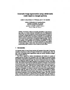
6.44 Histogram of reconstructed Fred image through CLRS

103

6.45 Histogram of reconstructed Fred image through PDAM

103

6.46 Histogram of the difference in pixels of reconstructed Fred image through CLRS and original Fred image

104

6.47 Enlarged histogram of the difference in pixels (Fred image reconstructed through CLRS)

104

6.48 Histogram of the difference of pixels of reconstructed Fred image through PDAM and the original image ( Fred)

105

6.49 Enlargement of the difference in pixels histogram (Fred image reconstructed through PDAM). Note that both x and y axis are modified.

105

6.50 Difference in pixel values. (Top) Difference between original Fred image and image enhanced by CLRS. (Bottom) Difference between original Fred image and image enhanced by PDAM.

106

6.51 Histogram of the normahzed fractal dimension of the Fred image

107

6.52 Enlarged histogram of the normalized fractal dimension of the Fred image.

107

X

6.53 Edges at different thresholds. (Top) Edges at a threshold of 233. after the fractal dimension of the Fred image was normalized within the range of 0 to 255. (Bottom) For the same normalized image edges at a threshold of 237.

108

6.54 Combination of processed images. (Top) Normalized fractal dimension of Fred image, first smoothed with PDAM and then thresholded at 232. (Bottom) The abo\e image combined with bottom center of image enhanced through CLRS. Note the highhghting and clear details. 109 6.55 Combination of edges. (Top) Sobel operator applied on Fred image with Ti = 20.$1 = 20. and gradient magnitude of 78. (Bottom) Bottom image reproduced from previous page for comparison purposes. 110 6.56 The Lubbock image and its processed output. (Top left) Original image of the city of Lubbock. (Top right) Image enhanced through CLRS using a = 0.2. A' = 0.2. i = 0.2. O, = C\. = 0.009.// = 0.8. (Bottom left) Edges at Q = 0.2. K = 0.2. ,i = 0 . 2 . 0 , = C, = 0.001.c^' = 0.8. (Bottom right) a = 0.2. K = 0.2. i = 0.2. Ch = C, = 0.08.7/ = 0.8.

Ill

6.57 Defective wafer image and its processed output. (Top) Original defective wafer image. (Bottom) Line process using CLRS after 7 iterationsll2 6.58 The wafer image processed through CLRS. (Top) Restored image through CLRS. (Bottom) State of the line process field after 1 iteration. 113 6.59 Processed wafer image. (Top) Defecti\'e wafer image processed through the PDAM. (Bottom) Image enhanced with CLRS using Q = 0.2. A' = 0.2. 3 = 2.0. O, = C, = 0.0001.7/ = 0.8 after 11 iterations. 114 6.60 Combination of processed output. (Top) Edges on a defective wafer image with simulated hard edges. The steps involved were (1) smoothing through CLRS with parameters Q = 0.2. 3 = 0.2, A' = 2.Ch = Cy = 0.0001.Lc' = 0.8 and (2) the resultant enhanced image was input to Sobel operator and then edge linked. (Bottom) Edges on a defected wafer image detected through Sobel operator, without first smoothing through CLRS.

115

6.61 Histogram of the normalized fractal dimension of the defective wafer image with an artificial hard edge

116

XI

6.62 Enlarged histogram of the normalized fractal dimension of the defective wafer image with an artificial hard edge.

116

6.63 Fractal dimension output of the wafer image. (Top) Normalized defective wafer image thresholded at 236. (Bottom) The same image thresholded at 240.

117

6.64 Fractal dimension output of the wafer image. (Top) Fractal dimension of the smoothed image thresholded at 237. (Bottom) Fractal dimension of the smoothed image thresholded at 241.

118

6.65 Fractal dimension output of the wafer image. (Top) Normalized fractal dimension output thresholded at 237 for defective wafer image (Bottom) The same image thresholded at 241.

119

6.66 Fractal dimension output of the wafer image. (Top) Fractal dimension of the smoothed image thresholded at 236 (Bottom) Fractal dimension of the smoothed image thresholded at 240.

120

6.67 Processed wafer image. (Top) Image enhanced through CLRS. (Bottom) Fractal dimension of the image given on top thresholded

121

6.68 Images processed with the Sobe operator. (Top) Sobel and edge linking on Fred image 20, 20, 80. (Bottom) Sobel and edge linking on defected wafer image with a simulated hard edge in it.

122

A.l Koch curve for four scales of magnification

140

Xll

CHAPTER I INTRODUCTION

Image restoration deals with the problem of reconstruction or estimation of the uncorrupted image from a distorted or a noisy image. The interest in this area is dri^•en by the application of restoration and segmentation to a wide variety of fields nameh- the earlv vision svstem. desisin automation, manufacturing; automation, vehicle guidance, archaeology, surveillance, and intelligent robots. In recent years many researchers[1]. [22]. [23]. [29] have investigated the reconstruction problem based on the Bayesian framework. In this framework, there are two models: (1) a prior model with probability distribution p(f) and (2) a measurement model with coiiditional distribution p(g/f). Here f denotes the estimate of the surface to be estimated and g denotes the observed values. Using Bayes rule posterior distribution p(f/g) can be obtained. The posterior estimate p(17g) is the likelihood of a solution f given the data g. If f is formulated as a Markov Random Field, then from Clifford-Hammersley theorem [5]. f can be descril)ed by a probability distribution of the Gibbs form. From the probability distribution p(f/g). f can be estimated in various ways. Marroquin [22] uses the maximum a posteriori (MAP) estimate, which maximizes p(f/g) and coincides with the minimum of a cost function. Geman and Geman [29] use simulated annealing to obtain the value of the estimate f. Blake and Zisserman [3]. using a model akin to

the deflection theory of thin plates, formulate a non-con^'ex. non-quadratic energy function and use a deterministic method, the Graduated NonCon^•exity (GNC) algorithm to find the minimum of an energy function. Terzopoulos[12] proposes a reconstruction method using a quadratic functional, which requires the solution of a single linear system to find the unique minimum. The methods outlined above are based on calculus of variations and mathematical statistics and do not directly incorporate the observed principles of low level animal vision. Linsker"s[6] studies on early stages of visual system show that networks developed on very simple biological principles develop optimization properties and hence may be utilized for finding the minimum of a cost function. Since many of the basic principles of low level mammalian visual system are now being understood, it may be worthwhile to apply these principles to machine restoration and segmentation of images. In this study, two major organizing principles of functional architecture of mammalian primaiy visual cortex: (1) Competitive learning and (2) Hebb type learning [9] are applied to image restoration. The principle of competitive learning is derived from the frequentl}* observed abilit}- of preserving neighborhood relations in feature maps in real brains [4. 9. 10] as signals are transformed over connections from the sense organs (e}^e. ear, skin) to the cortex and over connections between different areas of the cortex. Linsker [4] has reported that networks developed according to Hebb type rules develop response properties which are ^'ery similar to

3 mammalian visual system. Based on this, he has developed a theory of modular self-adaptive networks incorporating simple basic mechanisms by which feature analyzing functions observed in visual systems emerge. This theory, modified by neighborhood preserving assumptions, is extended in this work to formulate a Bayesian method of restoring degraded images. Simplifications result from the assumption that observations lie in a Markov Random Field (MRF). since computations can thus be restricted to immediate neighborhoods. In particular, the tea trade model [16. 17. 25] of competitive learning is extended for application to restoration of degraded image structures. In the tea-trade model, tea traders from India, each having a special blend of tea from his home town, delivers tea to traders in Britain. Traders in Britain make up their own blend by combining the tea delivered to them from different traders. After each trip to Britain, the traders from India adjust the quantity of tea to be delivered, based on their own and the customers blend. The dynamics of the trade is that the traders bring more tea for those customers, whose taste is closer to their own taste, as found in the previous trip. In earlier work [16]. the tea trade model has been effectively applied to other optimization problems, like the traveling salesman problem, for order of magnitude improvements in the speed of optimization relative to classical methods. Using the above principles of modeling a network for image segmentation and restoration, we have developed, implemented, and evaluated an iterative algorithm for simultaneous global matching of the observations to a given image. For future

reference, this algorithm will be called "Competitive Learning for image Restoration and Segmentation (CLRS)" algorithm. The image, which is represented by triplet>^ over a lattice, has three MRF"s: the intensity (F). horizontal discontinuity (H). vertical discontinuity {V). corresponding to each pixel in the lattice. The Markovian assumption allows the definition of image restoration techniques based on local interactions. The image restoration problem can thus be reduced to a minimization problem MiuEo{{F.H.

^')\g). where £"0 is a suitable energy function and g is the

measured value of image intensity. This work builds upon the work of Geman and Geman [29] and Durbin and Wilshaw [16]. The energ}* function chosen is unique in the sense that it is based on coefficients which measure how stronglv the intensitv f at a lattice point on the image is pulled towards a measured value g. thus successi^•ely matching the best overall fit to the total image. Estimation parameters are selected such that large adjustments occur earh' and are followed by later refinements. Restoration results of the CLRS algorithm are compared with restoration results of the model given by Geiger and Girosi [1], herein called PDAM (Parallel and Deterministic Algorithms from MRF"s). The underlying principle of this model is that the probability distribution of the configuration of fields, given a set of data, is a Gibb's distribution. Mean field approximation is used to find the mean value of the fields. The solution of the resulting deterministic equations is faster than the Monte Carlo techniques like simulated annealing, can be fully parallelized, and can

be implemented on analog networks. Geiger and Girosi [1] ha\-e reported ^•ery good restoration and segmentation results using this algorithm. From a conceptual viewpoint, it is better to smooth and do edge detection

A

simultaneously rather than smoothing and then edge detecting, since smoothing ;v ^^rt'^-^ first tends to remove the discontinuities that one tries to find in the edge detection phase. Both the algorithms, the PDAM algorithm and the CLRS algorithm simultaneously enhance the edges and smooth: incorporate the prior knowledge

/ ::,»raj^^/

about the surface: and account for the geometry of discontinuities. Geiger and Girosi show that it is essential for good cpialit}- restoration that edge detection and enhancement be done while smoothing is taking place. In our experiments on wide variety of synthetic and real images, both of these algorithms have shown ver}' good restoration and segmentation results. The edge maps produced using these algorithms are excellent representation of the image edges. In addition, both of these algorithms are rol^ust to the image structure and image quality. The segmentation results of the CLRS algorithm are compared with segmentation results of PDAM. the segmentation results using fractal dimension. \ ' and the segmentation results using the Sobel operator. A brief description of segmentation using the fractal dimension and segmentation using the Sobel operator is given in the following paragraphs.

*

T

6 Fractals [36] have a sound mathematical l^asis and form an important base for modeling many natural phenomena and engineering processes. Following on Mandelbrodt's work [36]. Pentland [35] has shown that the fractal dimension is a capable representation of succinctly describing the surfaces of natural objects such as mountains, trees, and clouds. Thresholding the histogram of the fractal dimension is used to segment the images. This approach gives vevy good results in segmenting regions with slowly changing intensity values, called soft edges, as opposed to edges that are a result of abrupt changes in the image intensity, which are called hard edges. Results reported in this work include a case where this method was able to detect fine boundaries. These boundaries were missed in segmentation results of all other approaches given in this work. Most common of the gradient operators is the Sobel operator [39]. Application of this operator gives a gradient image, which contains information about the magnitude and direction of change. Information from thresholding these quantities is used to link the edge points. These edge points were linked using a 3X3 mask around each edge point. In restoration techniques, preservation and enhancement of edges is a very important factor for overall quality improvement. The measures introduced by Abdou and Pratt [32]. and by Fram and Deutsch [33]. deal with edge detection schemes only, and do not take into account the schemes which simultaneously enhance and segment the images. In addition, these measures are edge detection

measures and do not measure the edge preservation and edge enhancement capability. We present a set of quantitative measures of image enhancement for synthetic images. These measures include edge enhancement and edge preservation measures for synthetic images. These measures are then used to compare the performance of the two algorithms, the CLRS and the PDAM. on synthetic images. To e^•aluate the performance of the CLRS and the PDAM. a set of two synthetic step images were generated. Gaussian and uniform noise was then added to each of the image. These corrupted images are then restored using CLRS and PDAM. For these synthetic images numerical measures developed in section 4.3.1 form the basis of comparison. All the four methods: the CLRS, the PDAM. segmentation using fractal dimension, and the Sobel operator were applied to a set of real images. On corrupted synthetic images, both techniques, the CLRS and PDAM. result in excellent performance. Based on numerical measures developed in section 4.3.1. PDAM is better in restoration, while CLRS is better in edge preservation and edge enhancement. On defective wafer image. CTRS seems to perform better than PDAM. Based on the analysis of results on synthetic and real images, both methods the CLRS and the PDAM seem to have equally good performance. Edge detection using fractal dimension was able to capture soft edges which were missed by CLRS. PDAM. and the Sobel operator. In general, combinations of edge maps from fractal dimension with any of these techniques gives discernible structural details and segments.

8 In summary, a new algorithm for image enhancement and edge detection is developed, implemented, and compared to a recently published algorithm using mean field approximation (PD.AM). as well as with the edge detection using the fractal dimension, and edge detection using the Sobel operator. A set of quantitative measures of performance are introduced. These measures form the basis of comparison of the algorithms the CLRS and PDAM for restoration of synthetic images. The performance of the CLRS. the PDAM. the fractal dimension. and the Sobel operator is compared on real images. The output of fractal analysis on real images is combined with the edge detected output of the other techniques. This in\'estigation. although preliminary, suggests a strong potential for improved segmentation. This dissertation is organized as follows. Chapter II gi^es the definitions and sets up the basic framework. Formulation and development of the CLRS algorithm is gi\-en in Chapter III. Chapter IV describes the PDAM model, the edge detection scheme using fractal dimension, and the Sobel operator. Section 4.3.1 gives the quantitati^'e measures of performance developed and used in this study. Chapter \ ' gives the structure of images and the noise model used in this study. Chapter M gives results obtained by processing the sample of images, and Chapter VII gi\es the conclusions and the suggestions for future work.

CHAPTER II FRAMEWORK AND METHODOLOGY

In this chapter, we give the basic definitions, introduce the terminolog}' used throughout the dissertation, and set up the background and framework for the development of the models: (1) the CLRS and (2) the PDAM.

2.1 Definitions and Framework In this study a surface is represented as a field, defined on a regular two dimensional lattice of sites. The value of this field at each site is given by surface height or intensity value at that site. The estimate of this surface consists of the intensity field, and two other fields the horizontal and vertical line processes (Figure 2.1). Let Z•n^n = { ( ^ j ) '• 1 ^ ' < 777.1 < j < ii} deiiote the mxn integer lattice of points. Given a neighborhood system [29] ^ = {^i^j.ii.j)

€ 2'„,„} on Zmn- where

>^ij ^ Z„^n denotes the neighbors of point (i. j). The neighborhood of a pixel selected in this work is comprised of four nearest neighbors (Figure 2.2). The neighbors of point (i,j) are the four points (? - 1. j ) , (?. j - 1). (i. j + 1). (? + 1. j ) [26]. We define a clique set A',j as a set of sites such that all the sites that belong to Xij are neighbors of each other.

10

1+2^+2

horizontal Geld (line process)

i'h2J-h2

Lattice

Figure 2.1: The surface field F, the horizontal line process H, and the vertical line process V are represented in two sites, (i.j) and (i-f2, j+2). of the lattice. Reproduced from [1].

,^ I V ^

J

iV!L

'^;>W-v

'^^

1.J

o

#

o

^ ("/>

Figure 2.2: The neighbors of point (i. j) are shown in dark circles.

i-l.j

ij

i,j+l

1.J

1.J

i+lj 1.J

iJ-1

Figure 2.3: Clique set for the pixel (i. j).

1.J

11

12 More formally. Definition 2.1.1 .4 clique set of the pair(Zmn-^)

denoted by Xij. /> defined a-

follows • A,/ consists of the single pixel {i.j).

• .for {i.j) 7^ {k.l).{i.j)

or

e Nij and {k.l) € A',, implies that {i.j) € 3^-/.

The clicpie set for the above neighborhood is shown in Figure 2.3. The importance of the clique structure is due to the fact that in the Gibb"s distribution, which forms an important base of this work, a sum is taken over potential energy terms. The potential energy is an interaction among pixels in the same clique. If the neighborhood, free to choice, is made larger than that used h e r e . ^ the clique structure grows very rapidh". For larger neighborhoods^the interactions over the pixels gets very complex. Definition 2.1.2 .4 line process field (edge element) is a binary valued rariable marking the presence (1) or absence (0) of discontinuity between intensity values at ^ adjacent pi.rel positions.

The horizontal edge element h,j denotes a discontinuity

marking unit between pi.rel position {i.j — 1) and {i.j). Vij denotes a discontinuity

The vertical edge element

marking unit between pixel positions {i — I.j)

and

{i.j)

(Figure 2.1). These selections are consistent with the clique structure given above. In this study, we model the image as a triplet F = {F. H.\

) . where F is the

matrix of pixel intensities. H and U correspond to the matrix of horizontal and

13 vertical edge elements. Thus. F is referred to as an intensity process. H as horizontal line process, and U as vertical line process, i.e. / . /?. r are the reahzations of the processes F. H. V. Following the terminology of [29]. we define F as

F

=

{.f,,}.(/.j)€Z^„.

(2.1)

Lowercase letters will denote the values assumed bv these random variables. Thus

{F = / } {H = h} {U = r }

stands for

{F,, = /,,. (K j ) € Zmn}-

(2.2)

stands for

{H,j = /?,,. {i.j) € Zmn}.

(2.3)

{Uj = f'o-(?• j ) € Z„,„}.

(2.4)

stands for

We model F.H. and U as MRF"s. i.e.. given a neighborhood system Ai an MRF over {Zmrn-^)

i^ ^ stocliastic process indexed by Zmrn foi' which

P{Frj=fij\F,l =

fu.{l^^-l)i^{^-j))

P{F,j = fij\Fki = A/. (A^ /) € ^,j).

P{H,,=li,j\Hu =

=

=

F{H,j=h,j\Hki

(2.5)

hki.{k.l)^{i.j)) = hu.{f^^-l)^^:j)-

(2.6)

14

Piyij

= v>j\^'ki =

v„.{k.i)j^{i.j))

= P{v>j = vi,\v,i = v,,.{k.i)e:s,,).

(2.7)

The Markov property- outlined above permits us to • use priors with neighborhoods that are small enough to ensure feasible computational loads and still rich enough to model and restore interesting classes of images.

• formulate a graph structure that has local characteristics.

• simultaneously update the line and pixel sites, and to

• restrict communication between pixels to neighbors only. Using the equivalence of MRF and Gibbs distribution, we formulate the restoration technique as a minimization problem [29] of the form minfE{{F.

H. '\')/g).

in which the problem is to find the image triplet {F. H. U).

which minimizes an objective function E. The measured image g is assumed to be known. The basic framework is Bayesian consisting of three MRF's: an intensity {F). horizontal discontinuity {H). and a vertical discontinuity (U) (Figure 2.1) [1]. hence we can define the svstem bv local interactions and capture the features of interest

15 by simply adding the appropriate terms in the cost function. Let the collection of fields {F.H.\')

be given by F . then according to Bayes theorem.

Pis) where the collection of field F and the input data are considered random variables. To make the connection to the Gibb's distril^ution. we need the following theorem. This theorem is used in the derivation of PDAM. T h e o r e m 2.1.1 Let ^ be a neighborhood system defined over the lattice Z. then a random field F = {/,j} defined on Z. has a Gibb's distribution or equivalently a Gibb's random field with respect to ^. iff its joint distribution is of the form

P{F = f)

where U{{f])

=

ie-^'(f-^»

= E.v'^ A-({/})- anfl U is an energy function,

(2.9)

and Uv({/}) is the

potential associated with clique N. and Z = E/^"^^"^^ '-^ ^^^^ partition function. partition function

is a normalization

The

constant and is the sum over all possible

configurations of F. The proof of the above theorem can be found in [13]. This theorem makes clear the necessity of keeping the neighborhoods small. For the choice of 4-nearest-neighbors and the resulting clique structure the potential terms for the Gibbs distribution are simply the pairwise interactions of the {i.j) pixel under

16 consideration with its 4-nearest-neighbors and with itself. Hence the sum over the clique structure can be simplified to a sum over just {i.j) and its nearest neighl)ors. The posterior estimate is the likelihood_^of the solution fij given the data g,j. The reconstruction problem can then be solved by finding an estimate f,j that either maximizes this Hkelihood (maximum aposteriori estimate) or minimizes the expected value of an error function with respectjo p{fjg).

Details of the CTRS

algorithm are given in section 3.1. and of PDAM algorithm are given in section 4.1.

2.1.1 Competitive Learning. Kohonens Algorithm In this section a brief description of competitive learning and Kohonen's algorithm is given. The leak}' learning form of the competiti\'e learning is used to develop the CLRS model, and the CLRS model is shown to have relationship with Kohonen"s algorithm (see chapter III).

2.1.1.1 Competitive Learning Let i''' be an input to a network of two layers with an associated set of weights iVi,. The standard competitive learning rule [11]. is given by

Ait>,

=

7/(^;-«>,).

(2.10)

which moves Wj. towards ,j+i - ^kj + .f>-i.j + .f>^i,jf-^/

(3.7)

mk

Hence EQ is a Lyapunov function. The coefficients A((?. j ) . (?77. A"). A') specify how strongly fij is pulled towards gij. 3. K take care of keeping fij's close to one another. The ratio of a to 3 controls the relative strength of the two terms. Since the update rule is of the form A/,j = ~^]j^.'

change in fij according to

the above update rule results in the reduction in the value of AQ. and since EQ is iDounded below, minimum of EQ will eventually be reached.

3.1.3 Relationship with Kohonen's algorithm Although the network structure of this model is different than the Kohonen's model, a formal relationship is shown to exist between the two. For the purpose of comparison, we rewrite Kohonens learning rule from equation 2.13

AWi

=

7//?(7.7")(v-Wr"''^).

25 Comparing equation (3.4) with Kohonen's rule given above, we find that a\{{i.j).

{m. k). K) plays the role of ///?(/. /') in Kohonen's learning rule.

The vector v in Kohonen's rule is replaced by its two-dimensional counterpart { gij }. Instead of wj. we modify / / / s in a Hebb-type learning rule. The s}naptic strength between neuron at position {i.j) € M and {i.j) e L is given by fij. Further, in Kohonen's rule h{i. i") is an adjustment function of the distance between the physical position of the two neurons, whereas in equation (3.4). \{{i.j).{iii.k).K)

is a measure of difference in intensity levels at position {i.j) in M

and position {m.k) in L.

3.1.3.1 Piecewise Smooth Surface Reconstruction The method outlined in the previous section smoothes over edges and thus fails to detect discontinuities. Now the line process field /, is introduced in the energy function. This indicates the presence or absence of discontinuity. (As discussed earlier, in two dimensions we have two line processes: one indicating a horizontal discontinuity (H). and the other indicating a vertical discontinuity (V)). The presence of discontinuities make the energy function nonconvex. Hence, the search space now includes many minima. In one dimension the energy function is given by

E = -aA'l^lnJ^e-^^'-^')' .

26

+ A^/,.

(3.S)

L is now the weight to be given to the cost of creating a discontinuit}- at i. Here Cs, is the one-dimensional analog of the neighborhood ^,/ introduced earlier (section 2.1). Replacing the right most term in equation 3.7. with the energy term corresponding to the line process term (A/) ancl_the interaction term (A,), the I ^--^>

update rule is given b}'

Afij

4(^3^" ^' ^

=

^1 1

aY.M{^.j)-{m.k).K){gmk-.f.j) nik

OF,

OF

CO

6 -

•H Q 0) n)

4 -

4J

o

2 -

M 0)

^igy

04

i«_L

0 50

m^^H

-J.

100 150 200 Gray L e v e l

250

300

Figure 5.12; Enlarged histogram of Image 1 corrupted by 50% Uniform noise

6: 45 c o •H 4J

3 Si •H M

40 35 30

4J CO •H

25

Q 0)

m 4J

20

15

-

c o

10 -

M 0)

5 -

04

J.

0 0

50

100 150 200 Gray L e v e l

250

300

Figure 5.13: Histogram of Image 2 corrupted by 50 % Uniform noise 10 c o •H 4-»

3 £t

•H M 4J

m

8 6 -

•H Q 0)

m

4 -

4J

c 0) o

2 -

M 0)

ML

04

0

50

J.

100 150 200 Gray Level

250

300

Figure 5.14: Enlarged histogram of Image 2 corrupted by 50 % Uniform noise

CHAPTER VI RECONSTRUCTION AND LINE PROCESS FIELD

This chapter gives the results of application of the mean field approximation and the proposed model to the synthetic and real images. The results on edge detection on real images using fractal dimension and the Sobel operator are also given in this chapter.

6.1 Synthetic Images This section gives the results corresponding to synthetic images.

6.1.1 Reconstruction and Line Process Field Losing Mean Field Approximation (PDAM) A brief description of the restored images, the associated line process fields, the associated histograms, and the parameters used in the rstoration and segmentation process for synthetic images are given in the following description. Figure 6.1. Image 1 (which was corrupted by 100%^ Gaussian noise) restored and the associated line process field. The parameters used were u.^ = O.OOOS.o- = 2.0.// = 2.0.0 = 10000, ;3 = 0.0005. The algorithm converged in 125 iterations.

Figure 6.2. Image 2 (which was corrupted by 100% Gaussian noise) restored and the associated line process field. The parameters used were 68

69 ^' = 0.0005, a = 2.0,// = 2.0.'; = 7000, i = 0.0005. The algorithm converged in 213 iterations.

Figure 6.3. Image 1 (which was corrupted b}- 50% Uniform noise) restored and the associated line process field. The parameters used were ^^ = 0.0005. o- = 2.0.// = 2.0. - = 10000,/i = 0.0005. The algorithm converged in 461 iterations.

Figure 6.4. Image 2 (which was corrupted with 50% Uniform noise) restored and the associated line process field. The parameters used were ^' = 0.0003. a- = 2.0. // = 2.0. -. = 10000. 3 = 0.0005. The algorithm converged in 176 iterations.

Figure 6.5 (enlarged plot in Figure 6.6). Plot of E versus the number of iterations for the restoration of the image 1 corrupted with 100% Gaussian noise.

Figure 6.7 (enlarged plot in Figure 6.8). Plot of E versus the number of iterations for the restoration of image 2 corrupted with 100% Gaussian noise.

Figure 6.9 (enlarged plot in Figure 6.10). Plot of E versus the number of iterations for the restoration of the image 1 corrupted with 50% Uniform noise.

Figure 6.11 (enlarged plot in Figure 6.12). Plot of E versus the number of iterations for the restoration of the image 2 corrupted with 50% Uniform noise.

70 Figure 6.13 (enlarged plot in Figure 6.45). Histogram of reconstructed image 1 (which was corrupted by 100% Gaussian noise) and restored through PDAM.

Figure 6.15 (enlarged plot in Figure 6.16). Histogram of image 2 (which was corrupted by 100% Gaussian noise) and restored through PDAM.

Figure 6.17 (enlarged plot in Figure 6.18). Histogram of image 1 (which was corrupted by Uniform noise) and restored through PDAM.

Figure 6.19 (enlarged plot in Figure 6.20). Histogram of image 2 (which was corrupted by Uniform noise) and restored through PDAM.

71

Figure 6.1; Restored image 1 (Gaussian 100 %, noise)using PDAM model (left) and associated line process (right)

Figure 6.2; Restored image 2 (Gaussian 100% noise) using PDAM (left) and associated Hne process (right)

Figure 6.3; Restored image 1 (50% Uniform noise) using PDAM model (left) and associated line process (right)

Figure 6.4: Restored image 2 (50%^ Uniform noise) using PDAM (left) and associated line process (right)

7000 -

T

T

E—

6000 5000 4000 Ed

3000 • 2000 1000 • 0 '•

X

j_

20

40

j -

j .

X

J-

60 80 100 120 140 Iterations

Figure 6.5: Image 1, Plot between iterations versus E (Gaussian noise) 200

T

1

1

1

1

r

150 Ed

1^

1

20

40

L

60 80 100 120 140 Iterations

Fio"ure 6.6; Enlarged plot between iterations versus E (Gaussian noise. Image 1)

6000 5000 4000 a

3000 2000 1000 J_

0

0

50

X

X

100 150 Iterations

X

200

250

Figure 6.7: Image 2. Plot between iterations versus E (Gaussian noise)

u

50

100 150 Iterations

200

250

Figure 6.8: Image 2. enlarged plot between iterations versus E (Gaussian noise)

/o

u

0 50 100150200250300350400450500 Iterations

Figure 6.9; Image 1. Plot between iterations versus E (Uniform noise) -iUU

i

1

1

1

1

1

1

1

T

E —

a

150

-

100

-

50 n

^ " ^ 4 -

1

1

1

1

1

J

J

X. -

0 50 100150200250300350400450500 Iterations

Figure 6.10; Image 1. enlargement plot between iterations versus E (Uniform noise)

j-^^^:-fijf

lOlog.o

•{dB)

(G.l)

j:.j{f,j-f!)^n:i'-f!j)

Table 6.1; Comparison of two algorithms for images corrupted by uniform 50% noise Image 1 Image 2 7/'*'^" Iterations 7/"^"' Iterations PDAM 4.86 461 4.72 176 CLRS

3.80

34

3.00

145

Table 6.2; Comparison of two algorithms for images corrupted by Gaussian noise 100% noise Image 2 Image 1 7/"^"' Iterations j^new Iterations 3.64 213 PDAM 13.36 125 CLRS

3.44

31

2.25

139

94 The following Table 6.3 and Table 6.4 give the comparison of two algorithms when maximum of 7/"'"' is achieved for restoring s}'nthetic images corrupted by noise.

Table 6.3; Comparison of two algorithms for images corrupted b}' Uniform 50% noise Image 1 Image 2 7/"'" Iterations 7/"^" Iterations PDAM 11.92 110 4.73 140 CLRS

8.-59

2

3.9

5

Table 6.4: Comparison of two algorithms for images corrupted by Gaussian noise 100% noise Image 1 Image 2 i^neu' Iterations j^new Iterations PDAM 13.38 118 3.7 116 CLRS

8.06

2

3.09

7

The Table 6.5 and Table 6.6 give the standard deviation of grey le^'els within each of the regions of the two images

Table 6.5: Region-wise SD of reconstructed images, which were corrupted by Gaussian Noise Image 1 Image 2 Region I Region II Region I Region II Region III CLRS 2.02 10.61 4.42 7.19 45.48 PDAM 2.55 2.31 2.00 6.72 40.08

Table 6.6: Region-wise SD of reconstructed images, noise Image 1 Region I Region II Region I 5.17 2.27 10.33 CLRS 2.-58 PDAM 6.56 6.66

which were corrupted by Uniform Image 2 Region II 6.60 5.73

Region III 37.01 32.63

96 The Table 6.7 and Table 6.8 give the comparison of the two algorithms on the ability of detection and preservation of edges and edge strengths (see section 4.3.1).

Table 6.7; Comparison of two algorithms for image 1 corrupted by Gaussian 100% noise Sh

br-

PDAM

1.14

0.91

1.03

3.83

CLRS

0.21

3.39

1.8

9.55

bs

Table 6.8: Comparison of two algorithms for image 1 corrupted by I'niform 50% noise Sh

b.

'-'avg

bs

PDAM

3.13

4.46

3.79

10.20

CLRS

0.38

2.78

1..58

8.68

97 6.1.2.1 Analysis and Interpretation 1. When we compare the restoration of Image 1 (Figure 6.1. Figure 6.21) and Image 2 (Figure 6.2. Figure 6.22) (earlier corrupted by Gaussian noise), the algorithms seem to have performed differently. Restoration of PDAM appears to be better and edge preservation of CLRS seems to be better. Similar results hold for restoration of images corrupted by uniform noise. Refer to Table 6.1 and Table 6.2. 7]^^'^'fi is higher for PDAM than is 7/^;^'^ for CLRS for both the Gaussian and Uniform noise and for both images. Hence based on the numerical measures PDAM algorithm has performed better on the smoothing of s}'nthetic images than the CLRS algorithm. In case of Image 2 the 7/" Y*^ for the two algorithms is very close.

2. From Figure 6.5. Figure 6.7. Figure 6.9. Figure 6.11. Figure 6.25. Figure 6.27. Figure 6.29. Figure 6.31. we note that for both the algorithms, and for each of the cases of Gaussian and uniform noise, large scale adjustments have taken l^lace in the first few iterations and are followed by finer refinements later on. From Table 6.1 and Table 6.2 we note that CLRS has faster convergence for both the images: image 1 and Image 2. and for both the cases of uniform as well as Gaussian noise.

3. From Table 6.3 and Table 6.4. we note that CLRS reaches a higher 7/5'>;>^ at a much faster rate. This may suggest that when rjf-^'f^ starts decreasing, it may

be more advantageous to stop further iterations, or to readjust the parameter values for further refinement. Exploration of this aspect of the algorithm forms an area of further research.

4. The histogram of the reconstructed image 1 through PDAM is much more like the histogram of the original image (Figure 6.13. Figure 5.5) than the histogram of the corrupted image (Figure 5.7). There is more spread in the histogram of Image 1 reconstructed through CLRS (Figure 6.33). thereby implying that PDAM has performed better than CLRS. Similar results hold for reconstruction of images corrupted by uniform noise.

5. In case of Image 2. for restoration of Gaussian noise, the spread of pixel values for PDAM is much wider than that of CLRS (Figure 6.15. Figure 6.35). Similar results hold for the case of uniform noise. Thereby implying that CLRS has performed better than PDAM. Results on edge preservation and edge enhancement are mixed. 1. In Table 6.7. for Gaussian noise 6/, for PDAM is 1.14 and that for CLRS is 0.21 thereby implving that CLRS has performed better than PDAM. However 8^. for PDAM is 0.91. which is much less than by for CLRS (which is 3.39) implying that PDAM has performed better than CLRS. These results are corroborated by the visual appearance.

99 2. For Gaussian noise 6, for PDAM is 3.83 and that for CLRS is 9.55 thereb}implying that PDAM has performed better than CLRS.

3. For uniformly corrupted images all the three values bh.S^.bs are less than that of PDAM thereb}- implying that CLRS has performed invariably much better than PDAM. These results are corroborated b}' the visual appearance.

6.2 Real Images In the following pages results from the application of the CLRS algorithm, the PDAM algorithm, the Sobel operator, and the Fractal dimension to a set of real images are given. Results on the union of edges from CLRS and fractal dimension, as well as combination of image enhancement by one method, and then edge detection through another method are also given. The caption given below each figure lists the parameters used and the process in^'olved in the generation of the photograph gi\-en in the figure. These photographs (from Figure 6.41 to Figure 6.68) are then followed by an analysis of the results.

100

Figure 6.41: The Fred image and its processed output. (Top left) Original Fred Image. (Top right) Restored Fred image through PD.\M after 14 iterations. The parameters used were a; = 0.001. a = 2,fi = 4.-) = 361. 3 = 0.005, (Bottom center) Line process field for w = 0.001, a = 2, ^ = 4, -; = 700, 3 = 0.05.

101

Figure 6.42; Processed Fred image through CLRS. (Top) Restored Fred image through CLRS, a = 0.2. K = 0.2.3 = 2.0. Ch = C = 0.008,// = 0.5 for 11 iterations. (Bottom) The associated line process field. Line process was updated after 7 iterations.

102

co

•H 4J

3 X3 •H M J-) 00

•H Q

!

r

I

••

••-•

16 14 12 10

-

8 6 4

M

04

2 ._ i .

0

50

100 150 200 Gray Level

_

J

250

300

Figure 6.44; Histogram of reconstructed Fred image through CLRS

o •H 3 X5 .H M

4 -

4J CO •H Q

3 -

0) C7^

1

1

1

i

'

•

1

25

3 Xi •H U V CO •H Q

20 15

3 X3 -H U 4J CO -H Q

0.12 -

0)

0.06 -



d 0)

o u

^ /o^(3") log4: log'i 1.26

140

Figure A.l: Koch curve for four scales of magnification