Proceedings of SPIE -- Volume 4476 Vision Geometry X, Longin J. Latecki, David M. Mount, Angela Y. Wu, Robert A. Melter, Editors, November 2001, pp. 186-193
Image Rectification Based on Minimal Epipolar Distortion∗ Zezhi CHEN **ab Chengke WU a and Li TANG a a
b
ISN National Key Lab., Xidian University, 710071, Xi’an , P.R.China Dept. of Computer, Xi’an University of Science & Technology, 710054, Xi’an, P.R.China ABSTRACT
This paper gives a new method for the rectification. The method is based on an examination of the fundamental matrix, which describes the epipolar geometry of the image pair. The approach avoids camera calibration and makes the resampling images extremely simple by using Bresenham Algorithm to extract pixels along the corresponding epipolar line. For a large set of camera motions, remapping to a plane has the drawback of creating rectified images that are potentially infinitely large and presents a loss of pixel information along epipolar lines. In contrast, our method guarantees that the rectified images are bounded for all possible camera motions and minimizes the loss of pixel information along epipolar lines. Furthermore, it never splits the image so that connected regions are no longer connected even if the epipole locates in the image. A large number of intensive experiments have been carried out, and the results show that more accurate matches can be obtained for initial pair of images after the rectification. Key words: Rectification, disparity, epipolar constraint, transformation, epipolar distortion, uncalibrated image.
1. INTRODUCTION Rectification is a necessary step of stereoscopic analysis. The process extracts epipolar lines and realigns them horizontally into a new rectified image with the epipolar lines coinciding with the image scan line. The epipolar lines run parallel with the x-axis and consequently, disparities between the images are in the x-direction only. This allows subsequent stereoscopic analysis algorithms to easily take advantage of the epipolar constraint and reduce the search space to one dimension, along the horizontal row of the rectified images
1, 2
.
The traditional rectification scheme consists of transforming the image planes so that the corresponding space planes 3
are coinciding . This is however not possible when the epipole is located in the image. Even when this is not the case the image can still become very big (i.e. if the epipole is close to the image). This is the reason why Roy. Meunier and 4
Cox proposed a cylindrical rectification scheme . The procedure described in there however, is relatively complex and 5
some important implementation details were not discussed. Hartely , begins to consider the problem of obtaining matched point between pairs of images, and develops further the method of applying projective geometric, calibrationfree methods to the stereo problem. But the intention is to resample the two images according to matching projective transformation F and F’, taking account of the fact that the matching projective transformation F and F’ have multiple results in general. If a projective transformation is a naughty productivity, it is possible to split the image so that connected regions are no longer connected. The method developed in this paper is a very simple algorithm for rectification, which works optimally in all possible cases, and it only requires the fundamental matrix between the two images. This method resamples two images by using Bresenham Algorithm extracting pixels along the corresponding epipolar lines. The image rectification method described here overcomes problem by transforming both images to a common reference frame, such as perspective distortion and resample distortion. Furthermore, it never split the image so that connected regions are no longer connected. This method may be used as a preliminary step to comprehensive image matching, and greatly simplifying the image-matching problem. Because we are effectively dealing with a rectilinear stereo frame, the mathematics of this reconstruction is extremely simple, and the resampled images are as good as the original ones. A large number of
* This project was supported by the Chinese National Natural Science Foundation, France-China Advanced Research Program and Hong Kong RGC grant. **
[email protected]; phone 86-29-8203116; fax 86-29-8232281
Part of the SPIE Conference on Vision Geometry X ● San Diego, California ● July 2001 SPIE Vol.4476 ● 0277-786X/01/$10.00
186
intensive experiments have been carried out, and the results show that more accurate matches can be obtained for initial pair of images after the rectification. This paper is organized as fellows. In Section 2, introduce the epipolar geometry constraint. In Section 3, Determining the common region, and resampling the rectified images by using Bresenham Algorithm extract pixels alone the epipolar line. In Section 4, algorithm outline is summarized. The experimental results shown in Section 5 and the conclusions are given in Section 6.
2. EPIPOLAR GEOMETRY CONSTRAINT Suppose two images are acquired of a 3D scene, with two cameras (or a single camera moving) related by a rotation and non-zero translation. An image point mi in the first view corresponds to an image point mi ' in the second if they are images of the same 3D point. The epipolar geometry constraint describes the relations that exist between two images. Every point in a plane that passes through both centers of projection will be projected in each image on the intersection of this plane with the corresponding image plane. Therefore these two intersection lines are said to be epipolar correspondence. This geometry constraint can easily be robust recovered from the image pairs constraint, we have
6−11
. From the epipolar geometry
m 'T Fm = 0 F e = F T e' = 0
(1)
(2) where m and m’ are the perspective projection points of a 3D point M, with their homogenous coordinates being
( x, y,1) T and ( x' , y ' ,1) T , respectively. The fundamental matrix F is a 3× 3 matrix, which maps a point m in image 1 to its corresponding epipolar line l ' ~ Fm in image 2. This matrix has rank two (~ meaning equality up to a non-zero scale factor). The fundamental matrix has only seven degrees of freedom. Thus, in order to estimate fundamental matrix, seven pairs matching points mi ↔ mi ' between the two images are at least needed. If we have 8 matching points, the improved 8-point algorithm be used.
12
can be used. If we have more than 8 matching points, the nonlinear iterative method can
3. RECTIFICATION Determining the common region. Before determining the common epipolar lines, the extreme epipolar lines for a single image should be determined. These are the epipolar lines that touch the outer image corners. The different regions for the position of the epipole are given in Figure 1. 1
A
D 3
5
4
7
2
B
8
6 C
9
Figure 1. The extreme epipolar lines can easily be determined depending on the location of the epipole in one of the 9 regions. The image corners are given by A, B, C, and D
The extreme epipolar lines always pass through corners of the image. e.g. If the epipole is in region 1 the area between eB and eD, if the epipole is in region 3 the area between eA and eC, etc. The extreme epipolar lines from the second image can be obtained through the same procedure. The common region is then easily determining as in Figure 2.
187
e
e' E
I
H
F
l1'
E'
l1
I'
l3
l3 '
F'
G
G'
l2
H'
l2 '
l4 ' Figure 2. Determination of the common region. The extreme epipolar lines are used to determine the maximum angle. l4
m × n , then the corners A, B, C and D with their homogenous coordinates are (0,0,1) , (0, n,1) , (m, n,1) and (m,0,1) T , respectively. The epipolar line l 3 , l 4 , l1 ' and l 2 ' are given as We assumed that the image size is T
T
T
follows:
l1 ' ~ FA
l 2 ' ~ FC
l3 ~ F T A
l4 ~ FT C
(3)
l1 ' intersects the right border of the image 2, and the intersection out of the image 2, then the extreme upper epipolar line of the image 1 is l 3 . Otherwise, the extreme upper epipolar line of the image 1 is l1 . The extreme lower epipolar line of the image 1 can be obtained through the same where ~ meaning equality up to a non-zero scale factor. If the line
procedure. The common regions EFGHI in the image 1 and E’F’G’H’I’ in the image 2 can be obtained, respectively. Epipolar line transfer. To avoid losing pixel information, the area of every pixel should be at least preserved when transformed to the rectified image. The worst-case pixel is always located on the image border opposite to the epipole (i.e. the right border in Fig. 3). In Figure 3, e is the epipole in the image 1, l i is an arbitrary epipolar line. It intersects the left border at A and the right border at B. The line A’B’ is the epipolar line corresponding to AB, and it parallel to resample image scan lines. The coordinates of B’ are coinciding with B.
e A
li B
A'
li ' B'
Figure 3. Epipolar line transfer
In order to draw the epipolar line A’B’ and avoid pixels loss, every pixel along the line AB corresponding A’B’ can be 13
extracted by using Bresenham Algorithm . Drawing line AB and A’B’ is accomplished by calculating intermediate positions along the line path between two endpoint. An output device is then directed to fill in these positions between the endpoints. Figure 4 illustrates a section of a display screen where straight-line segment is to be drawn. The vertical axes show scan-line positions, and the horizontal axes identify pixel columns. So plotted positions may only approximate actual line positions between two specified endpoints.
188
Scan-line Number
Scan-line Number
x
x
B A' 0 1 2 3 4 5 6 7 8 9 10 11 12 13 14 15 16 17 18 19 20 21 22 23
Pixel column number
0 1 2 3 4
0 1 2 3 4
5 6 7
5 6 7
8 9
8 9
A
B' 0 1
2
3
4
y
5
6
7
8
9 10
11 12 13
14 15 16
17 18 19 20 21
22 23
y
Pixel column number
Figure 4. resample algorithm
In Figure 5,
l i −1 and l i are two consecutive epipolar lines. Let the coordinates of e is (e x , e y ) .
(
· the epipole e out of the image. When the epipole e is in the region 1(Fig. 5 (a)), and if e y + n
)
e x > 1 , let
extreme upper epipolar line of the common regions intersects the right border at C and the extreme lower epipolar line of the common regions intersects the bottom border at D. Then the start-point is C, and the end-point is D. Otherwise, the end-point is the intersection of the extreme lower epipolar line of the common regions with the right border E. Let l i −1 and l i intersect image border at A and B respectively. To avoid pixel loss, the distance AB should be at lest one pixel. In this case, the maximal height of rectified image is m+n. The same procedure can be carried out in other regions, such as region 3, 7, 9. When the epipole e is in the region 4(Fig. 5 (b)), and if e y
e x > 1 , then the start-point is the intersection of the
extreme upper epipolar line of the common regions with the top border C. Otherwise the start-point is the intersection of the extreme upper epipolar line with the right border D. If n − e y e x > 1 , then the end-point is the
(
)
intersection of the extreme lower epipolar line of the common regions with the bottom border E. Otherwise the endpoint is the intersection of the extreme lower epipolar line with the right border F. To avoid pixel loss the distance AB should be at lest one pixel as well. In this case, the maximal height of rectified image is 2m+n. The same procedure can be carried out in other regions, such as region 2, 6, 8. · The epipole e is locate in the image. If the epipole is in the image an arbitray epipolar line can be chosen as starting point. In this case boundary effects can be avoided by adding an overlap of the size of the matching window of the stereo algorithm. Let
l i −1 and l i intersect four borders of image, the intersection are A and B, the distance AB
should also be at lest one pixel. In this case, the height of rectified image is 2(m+n) (Fig. 5 (c)). Resample the rectified image. To resample the rectified image, the first step consists of determining the common region for both images. Then, starting from one of the extreme epipolar lines, the rectified image is built up line by line. Each row corresponds to a certain angular sector, and the number of pixels along the epipolar line is preserved. So all pixels in the image are preserved and minimize the loss of pixel information along epipolar line. The same procedure can be carried out in the other image. In this case the obtained epipolar line should be transferred back to the first image. The minimum of both displacements is carried out. At the same time, the coordinates of every pixel along the epipolar line are saved in a list for later reference, i.e. transfer back to original images. Transferring information back. Information about a specific point in the original image can be obtained as follows. Every pixel in the rectified image corresponding to the unique pixel in the original image, so we can look up it pixel-bypixel in the list which have saved last paragraph.
189
e D
C l i −1
C l i −1 li
A B
li
e
l i −1
A B
li
e E
D
A B
F
E
(a)
(b)
(c)
Figure 5. Determining the minimum distance between two consecutive epipolar lines
4. ALGORITHM OUTLINE The rectification algorithm will now be summarized. The input is a pair of images containing a common overlap region, and the output is a pair of images resampled so that the epipolar lines in the two images are horizontal (parallel with the x-axis), and the epipolar lines coincide with scan line, such that corresponding points in the two images are as close to each other as possible. Any remaining disparity between matched points will be along the horizontal epipolar line. The algorithm outline generalized as follows. 1. Find at least seven matching points mi ↔ mi ' between the two images. 2. 3. 4. 5.
Estimate the fundamental matrix, and compute the epipoles e and e’ in the two images. Determine the common region by using epipolar geometry constraints. Transfer the epipolar line by using formula (3) and extract pixels by using Bresenham Algorithm. Resample the rectified image.
5. EXPERIMENTS A large number of real images were selected to measure performance. Two images taken from widely different relatively oblique viewing angles are shown in Figure 6. The resulting resampled images are shown side-by-side in Figure 7. As may be discerned, any disparities between the two images are parallel with the x-axis. Figure 8, 9 and Figure 10, 11 show other two pairs of images and its resulting resampled images. It is demonstrated that the method gives results superior to previous approaches.
Figure 6. a indoor scene and a few of epipolar lines
190
Figure 7. The resampled indoor scene and a few of epipolar lines
Figure 8 Two images of a building
Figure 9 The two resampled images of a building
191
Figure 10 two images of an old building
Figure 11 The two resampled images of an old building
6. CONCLUSION This paper gives a rapid practical algorithm for the rectification of stereo images take from widely different viewpoints. The method makes the computation of the scene geometry extremely simple. Furthermore, it minimizes the loss of pixel information along epipolar line and the resampling distortion. Because of the great simplicity of the epipolar transformation, the resampling of the images may be done extremely quickly.
ACKNOWLEDGEMENTS We wish to thank all those people who supplied real images for testing the algorithm presented in this paper.
REFERENCES 1.
W. Hoff and N. Ahuja, “Surfaces from stereo: Integrating feature matching, disparity estimation and contour detection,” IEEE trans. on Pattern Analysis and Machine Intelligence, vol. 11, no. 2. pp. 121-136, 1989.
192
2. 3. 4. 5. 6. 7. 8. 9. 10. 11. 12. 13.
M. S. Lew, T. S. Huang and K. Wong, “Learning and feature selection in stereo matching,” IEEE Trans. on Pattern Analysis and Machine Intelligence, vol.16, no. 9, pp. 869-881, 1994. D. V. Papadimitriou and T. J. Dennis, “Epipolar line estimation and rectification for stereo image pairs,” IEEE transaction on Image Processing, vol.5, no.4, pp.672-677, 1996. S. Roy, J. Meunier and I. Cox, “Cylindrical rectification to minimize epipolar distortion,” Proc. IEEE Conference on Computer Vision and Pattern Recognition, pp. 393-399, 1997. R. Hartley, “Theory and practice of projective rectification,” International Journal of Computer Vision, vol. 35, no. 2, pp. 115-127, 1999. Zezhi Chen, Chengke Wu, Peiyi Shen, Yong Liu, Long Quan, “A Robust Algorithm to estimate the Fundamental matrix,” Pattern Recognition Letters, vol. 21, pp. 851-861, 2000. O. Faugeras, Three-Dimensional Computer Vision: A Geometric Viewpoint, Cambridge, Massachusetts, London, England: The MIT Press, 1993. R. Hartley, “In defence of the 8-point algorithm,” In: Proceedings of the 5th ICCV, Cambridge, USA, pp.882-887, 1995. Zhang Zheng-You, “Determining the epipolar geometry and its uncertainty: a review,” International Journal of Computer Vision, vol. 27, no. 2, pp. 161-195, 1998. Q. T. Luong and O. D. Faugeras, “On the determination of epipoles using cross-ratios,” Computer Vision and Image Understanding, vol. 71, no. 1, pp. 1-18, 1998. Chen zezhi and Wu Chengke. “A weighted normalization method of estimating fundamental matrix and its stability analysis,” Chinese Journal of Electronics, vol. 9, no. 3, pp. 229-234, 2000. R. Hartley, “In defence of the 8-point algorithm,” In: Proceedings of the 5th ICCV, Cambridge, USA, pp.882-887, 1995. Donald Hearn and M. Pauline Baker, Computer Graphics, Second Edition, Prentice-Hall International Inc. Press, 1998.
193