ABSTRACT. Resampling techniques are commonly required in digital image processing systems. Many times the classical inter- polation functions are used, i.e., ...
IMAGE RESAMPLING BETWEEN ORTHOGONAL AND HEXAGONAL LATTICES Dimitri Van De Ville∗,1 , Rik Van de Walle1, Wilfried Philips 2, Ignace Lemahieu1 Ghent University – 1 E LIS, 2 T ELIN Sint-Pietersnieuwstraat 41 B-9000 Ghent, Belgium ABSTRACT Resampling techniques are commonly required in digital image processing systems. Many times the classical interpolation functions are used, i.e., nearest-neighbour interpolation and bilinear interpolation, which are prone to the introduction of undesirable artifacts due to aliasing such as moire patterns. This paper presents a novel approach which minimizes the loss of information, in a least-squares sense, while resampling between orthogonal and hexagonal lattices. Making use of an extension of 2D splines to hexagonal lattices, the proper reconstruction function is derived. Experimental results for a printing application demonstrate the feasibility of the proposed method and are compared against the classical techniques. 1. INTRODUCTION Digital images are sampled on a regular lattice. The conversion of this representation from one lattice to another is called image resampling. This operation is indispensable for many applications such as printing. We propose a new method to resample between orthogonal and hexagonal lattices. The standard procedure for linear resampling consists of two conceptual steps: first, an image in the continuous domain is reconstructed; second, this function is resampled on the target lattice [1, 2, 3, 4]. Shannon’s sampling theorem assumes that images are band-limited, and proposes to choose the interpolation filter to the ideal low-pass filter. However, real-world signals are not band-limited and both the image and the interpolation function have a finite support. Due to the slow decay of the ideal interpolation functions (which are sinc-like), it is also quite difficult to approximate them on a finite support. Additionally, ideal interpolators tend to generate the Gibb’s phenomenon, which becomes visually apparent in images as ringing along the edges. Instead of holding on to the band-limited hypothesis, many authors, such as Unser [5, 6, 7, 8], set up a family ∗ Dimitri Van De Ville is a Research Assistant with the FWO Flanders, Belgium
0-7803-7622-6/02/$17.00 ©2002 IEEE
of basis functions based on splines. These splines have a limited size of support, which expands as the order increases. Ultimately, a spline representation of infinite order approaches the ideal filter. For example, first-order spline interpolation is better known as “nearest neighbour” interpolation; second-order spline interpolation as bilinear interpolation. Higher orders, such as bicubic spline interpolation yield even smoother results. The standard approach does not minimize the information loss. Annoying artifacts due to aliasing (such as moire patterns) might arise. Unser et al. [5, 9] derived an algorithm based on the principle of convolution-based leastsquares spline approximation. In particular, the samples on the target lattice are chosen such that the mean squared error between the spline representation on the source lattice and a similar one on the target lattice is minimized. This theory was developed for a 1D spline representation, and extended to 2D orthogonal lattices by means of tensor-product splines (i.e., the 2D spline is the product of two 1D splines). This paper discusses the case of resampling between orthogonal and hexagonal lattices, therefore requiring a spline definition suitable for hexagonal lattices. We propose a simple recipe to construct hexagonal splines and make use of these splines to derive the least-squares reconstruction function. To demonstrate the feasibility of the proposed approach, we implemented our method for the practical case of gravure printing, a printing technique which is very susceptible to aliasing artifacts when using classical resampling procedures. 2. TWO-DIMENSIONAL SPLINES We will denote a 2D function in the continuous domain as g(x), where x ∈ �2 . The L2 -norm of g(x) is derived from the inner product: ||g|| = �g, g� 1/2 . Analogously, we denote a discrete 2D array as c(k), where k ∈ � 2. We denote �� �1/2 ∗ the l2 -norm of c(k) as ||c|| l2 = . k∈�2 c(k)c (k) A 2D lattice can be characterized by a matrix R = [r1 |r2 ] constituted of two linearly independent vectors r 1 and r2 [10]. It is convenient to define an array of impulses
III - 389
IEEE ICIP 2002
(a)
on the lattice sites: δR (x) =
� k∈
�
δ(x − Rk),
(1)
2 1
where δ(x) represents a Dirac function. Related to a lattice is a Voronoi cell, which is defined as the set of all points that are closer to the origin 0 than to any other site of the lattice. The Voronoi cell is represented by its indicator function χ R (x): x ∈ Voronoi cell, 1, χR (x) = 1/m, x on edge Voronoi cell, (2) 0, x∈ / Voronoi cell, where m equals the number of lattice sites to which x is equidistant. Note that this function, when periodically copied onto all the lattice sites, covers the complete plane: δR χR (x) = 1, where the -operator denotes the 2D continuous convolution. It is said that the Voronoi cell tiles the plane. Consider a function g(x), which is sampled on each lattice site of a lattice R. Using a shift-invariant 2D generating function φ(x), we define the approximation space S(φ) as follows [11]
� � c(k)φ(x − Rk) , (3) S(φ) = s(x) s(x) = k∈
�
2
where the coefficients c(k) need to be chosen such that s(Rk) = g(Rk). As such, any function s(x) ∈ S(φ) is characterized by a sequence of coefficients c(k). Notice that these coefficients are not necessarily samples s(Rk) at the lattice points. Several conditions are required to obtain a sensible continuous/discrete model [11], among which most importantly to form a Riesz basis. Splines suitable for a regular orthogonal lattice, described by the unity matrix, can easily be obtained by using the tensor-product of two one-dimensional B-splines β n (x) = β n (x1 )β n (x2 ). The superscript n refers to the n-th degree of piecewise polynomials or to the n + 1-th order of approximation [12]. Consider now a regular hexagonal lattice, described by � √ 3/2 0 ˜ R= . (4) −1/2 1 We define the√ surface area of the Voronoi cell as Ω = ˜ = 3/2. Matrices and functions related to the det(R) hexagonal lattice are denoted by the ˜-notation. To construct a spline basis on the hexagonal lattice, we are especially interested in preserving the convolution property because it plays an important role in the derivation of the least-squares approximation later on. Therefore, we first
0.8 0.6 0.4 0.2 2
0 2
1 1 0 0 −1
−1
x2
−2
x1
−2
(b)
1 0.8 0.6 0.4 0.2 2
0 2
1 1 0 0 −1
−1
x2
−2
−2
x1
Fig. 1. Splines derived on a hexagonal lattice. (a) First order, (b) Second order. define the first-order hexagonal spline as the indicator function of the Voronoi cell: β˜0 (x) = χR ˜ (x). Note that this spline is normalized to the surface area of the basic cell:
0 β˜ dx = Ω. By convolving this function with itself repeatedly, we construct hexagonal splines of higher orders: β˜0 β˜n−1 (x) , β˜n (x) = Ω
n ≥ 1.
(5)
Figure 1 shows the hexagonal splines of first and second order. The successive convolutions imply that the splines become smoother as the order increases. Interesting properties of the hexagonal splines (analytical form, Riesz basis, convexity, partition of unity, computation of the spline transform) can be found in [13]. 3. LEAST-SQUARES RESAMPLING Consider now two periodic lattices, i.e., an orthogonal ˜ The source lattice R and a hexagonal target lattice R. two-dimensional splines of the previous section allow us to easily reconstruct an image in the continuous domain, using a reconstruction of the approximation spaces S(β n ) and
III - 390
S(β˜n ). We are aiming at a convolution-based scheme g˜n (Rk) = s(Rk);
s(x) =
�
Φn (x−Rk)g(Rk), (6)
k
where the reconstruction function Φ n (x) realizes the leastsquares approximation between both spline reconstructions. The minimum L 2 -norm approximation of a function g(x) can be found by projection on S( β˜n ). As such, the error g(x) − g˜n (x) is orthogonal to S( β˜n ). Since the original function g(x) is only known at the lattice sites Rk, we replace g(x) by its approximation in S(β n ), using a spline model for the source lattice. This enables us to write ˜ = 0, �g n (x) − g˜n (x), β˜n (x − Rk)�
(7)
where g n (x) and g˜n (x) are the spline representations respectively on the orthogonal and hexagonal lattice. We can rewrite the expression as ˜ �g n (x), β˜n (x − Rk)� � ˜ ˜ = � c˜(k)β˜n (x − Rk), β˜n (x − Rk)�
Φ1 (x) = β 1 (˜b3 )−1 β˜1 (x)/Ω.
k
=
�
˜n
˜n
˜ ˜ c˜(k)�β (x − Rk), β (x − Rk)�,
(8)
k
where c˜(k) are the spline coefficients on the hexagonal lattice. We now use the founding property of the hexagonal splines β˜n β˜n (x)/Ω = β˜2n+1 (x): g n β˜n (x) = Ω
� �
� ˜ c(k) δ(x − Rk)˜
The computation of Eq. (11) requires the solution of two direct spline transforms (the inverse filters). One solution is to invert the matrix corresponding to the set of linear equations induced by the forward filters [7]. Another approach could be to implement the inversion scheme by means of recursive filters similar to the approach proposed by Unser [14, 6]. However, the factorization of the filter corresponding to the hexagonal splines is not trivial. Therefore, we propose to numerically approximate the reconstruction function on a limited support by means of a well-known iterative procedure [15]. In the case of n = 0, the reconstruction function of Eq. (11) becomes Φ 0 (x) = β 0 β˜0 (x)/Ω. No inverse filters are needed and the support is limited. This case is sometimes referred to as “surface projection”: neighbouring samples of the source lattice are weighted by the relative overlap of source’s and target’s cell. For the second-order least-squares approximation, the reconstruction function is given by
The presence of the inverse filter (˜b3 )−1 implicates that the theoretical support of Φ 1 (x) is the whole plane [13]. However, the fast decay shows that an approximation on a limited support is appropriate. Note that this approach can easily be applied to resampling from hexagonal to orthogonal lattices. In that case, the inverse filters can be computed by recursive filters given in [14].
β˜2n+1 (x). (9)
k
4. RESULTS
The solution of Eq. (8) can be written as c˜(k) =
g n β˜n (˜b2n+1 )−1 (Rk), Ω
(10)
where bn (x) = β n (x)δR (x) is the “sampled spline”. This enables us to write the least-squares interpolation function ˜ as for resampling from the lattice R to R ˜bn (x)/Ω, Φn (x) = (bn )−1 β n β˜n (˜b2n+1 )−1 ���� � �� � � �� � 1
(12)
2
We implemented the proposed resampling method for a gravure printing application. The images are resampled to a hexagonal lattice before halftoning. Figure 2 shows the results of a test image after resampling using classical interpolation functions in (a)-(b), and after least-squares resampling in (c)-(d). The corresponding reconstruction functions are depicted in (e)-(f). Kindly note that the moire patterns are better suppressed by the least-squares approach and the second order least-squares produces sharper results.
3
(11)
5. CONCLUSION
where the underbraced expressions indicate: 1. the direct spline transform to compute the spline coefficients on the source lattice; 2. the least-squares approximation filter; 3. the final convolution to reconstruct the function in S(β˜n ) using the new spline coefficients.
In this paper, we presented a new method to resample between orthogonal and hexagonal lattices. After proposing a simple recipe to derive a two-dimensional spline basis for hexagonal lattices, we applied the principle of a leastsquares approximation to derive a suitable reconstruction function. Many applications involving hexagonal lattices can make use of this approach.
III - 391
(a)
(c)
(e)
0.6 0.5 0.4 0.3 0.2 0.1 2
0 2
1 1 0 0 −1
−1
x2
(b)
(d)
−2
−2
x1
(f)
0.6 0.5 0.4 0.3 0.2 0.1 5
0 5 0 0
x2
−5
−5
x1
Fig. 2. Results after resampling the test image “shirt” to the gravure lattice. (a) Interpolative resampling (first order), (b) Interpolative resampling (second order), (c) Least-squares resampling (first order), (d) (Least-squares resampling (second order). (e) Reconstruction function for “surface projection” Φ 0 (x). (f) Reconstruction function Φ 1 (x). 6. REFERENCES
tics, Speech, and Signal Processing, vol. 26, no. 6, pp. 508– 517, Dec. 1978.
[1] A. Rosenfeld and A.C. Kak, Digital Picture Processing, Academic Press Inc., 2 edition, 1982.
[9] M. Unser and I. Daubechies, “On the approximation power of convolution-based least squares versus interpolation,” IEEE Transactions on Signal Processing, vol. 45, no. 7, pp. 1697–1711, July 1997.
[2] D.P. Mitchell and A.N. Netravali, “Reconstruction filters in computer graphics,” ACM Computer Graphics, vol. 22, no. 4, pp. 221–228, Aug. 1988.
[10] R.A. Ulichney, Digital Halftoning, MIT Press, 1987.
[3] J.C. Russ, The image processing handbook, CRC Press Inc., 1992.
[11] M. Unser, “Sampling—50 years after Shannon,” Proceedings of the IEEE, vol. 88, no. 4, pp. 569–587, Apr. 2000.
[4] R. Soininen, “Digital Image Resizing Methods,” M.S. thesis, Tampere University of Technology, 1994.
[12] P. Th´evenaz, T. Blu, and M. Unser, “Interpolation revisited,” IEEE Transactions on Medical Imaging, vol. 19, no. 7, pp. 739–758, July 2000.
[5] M. Unser, A. Aldroubi, and M. Eden, “Enlargement or reduction of digital images with minimum loss of information,” IEEE Transactions on Image Processing, vol. 4, no. 3, pp. 247–258, Mar. 1995. [6] M. Unser, A. Aldroubi, and M. Eden, “B-spline signal processing,” IEEE Transactions on Signal Processing, vol. 41, no. 2, pp. 821–848, Feb. 1993. [7] C. de Boor, A Practical Guide to Splines, vol. 27 of Applied Mathematical Sciences, Springer-Verlag, 1978. [8] H.S. Hou and H.C. Andrews, “Cubic splines for image interpolation and digital filtering,” IEEE Transactions on Acous-
[13] D. Van De Ville, W. Philips, and I. Lemahieu, “Least-squares spline resampling to a hexagonal lattice,” Signal Processing: Image Communication, accepted for publication. [14] M. Unser, “Fast B-spline transforms for continuous image representation and interpolation,” IEEE Transactions on Pattern Analysis and Machine Intelligence, vol. 13, no. 3, pp. 277–285, Mar. 1991. [15] R.W. Schafer, R.M. Mersereau, and M.A. Richards, “Constrained iterative restoration algorithms,” Proceedings of the IEEE, vol. 69, no. 4, pp. 432–450, Apr. 1981.
III - 392